Website powered by

Niagara Visualize Audio FX and Sample Submixes

Tutorial / 11 May 2023


Outline

  • Introduction

  • Particle System Initial Setup

  • Sample Audio

  • Sampled Value Uses Examples

  • Fade Sampled Audio

  • Sample from Custom Submix

  • Conclusion

---

Introduction

In this post I will cover some techniques I found useful when developing Niagara FX that reacts to audio, I made one that you can check out here → Equalizer FX - Niagara UE5
This post will cover a more simple setup, showing how you can create a basic Visualize Audio FX that can be useful for debugging purposes. One other thing I will also go over is how you can create your own custom Submix so that you can make the FX react only to the audio coming from a target Submix instead of using the built-in MasterSubmixDefault, which contains every sound that plays in the level.

The following video shows the final result of the Niagara System this tutorial will breakdown:

---

Particle System Initial Setup

Before starting to sample audio we need some particles. Below you can find the initial setup of the Emitter I've made and all the User Parameters I've exposed.

User Parameters

  • AudioOscilloscpe → target submix to sample audio from
  • AudioSpectrum → target submix to sample audio from
  • FadeSpeed → speed rate at which the sampled audio value should fade , explained in the "Fade Sampled Audio" section
  • isSpectrum → this is a boolean that switches the logic from using the AudioOscilloscope and the AudioSpectrum, two different methods to sample audio
  • VisualizerHeight → used to set the particles' height
  • VisualizerResolution → how many particles , which consequentially defines the resolution and precision of the sampled audio's visualization
  • VisualizerWidth → used to set the particles' width


Emitter Properties

The emitter is GPU based, make sure you set some Min and Max bounds


Emitter State

Life Cycle Mode is set to Self
Loop Behaviour to Once
Loop Duration Mode to Infinite


Spawn Particles in Grid

the particles are disposed on a horizontal line, to achieve this I've used Spawn Particles in Grid and Grid Location modules.
Y and Z Counts are set to 0, while X is defined by the VisualizerResolution User Parameter


Gird Location

The *Grid Location* module works hand-in-hand with the Spawn Particles in Grid.
There are some Z offset values, this is to move the particles up by half the size of the particles (defined by VisualizerHeight), doing so the particles will be placed above the Niagara System's Pivot Point.
For the Dimensions, I'm doing a simple operation on X so that the width's result perfectly matches the VisualizerWidth User Parameter in units. Using the VisualizerWidth value directly doesn't give a perfect result, it's going to be wider by one particle width.

What the X Dimensions fixes:
Before → the particles are wider than 256 units and there is a small gap between them


After → the particles perfectly match the 256 units in width and there is no gap between them


Initialize Particle

For the Initialize Particle module, the most important part is to set the Mesh Scale X and Z.
Z is simply using VisualizerHeight User Parameter, 
To calculate the correct size in X I'm dividing VisualizerWidth by VisualizerResolution.
Both of them are divided by 100 because the mesh used is 1x1x1 meter, the division gives us the value in millimeters.
I'm also doing a little trick on the colour just to get a random value for each particle and distinguish them from one to another.


Set Particles Attribute UVs

I made 3 custom Particle Attributes, the first one is a Vector2D and is called UVs.
This is a useful technique to get a 0-1 gradient value when using the Spawn Particles in Grid and Grid Location modules, they output a GridUVW value, which we can store in the particles.
In this FX I'm actually only using X, so you could store it to a Float instead of a Vector2D.

This is what you would get if the particles' colour was set to the U value


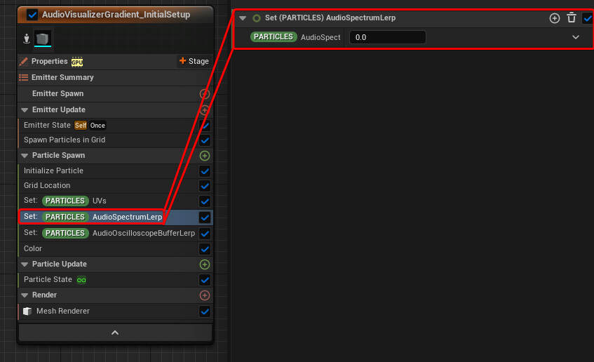
Set Particles Attribute AudioSpectrumLerp and AudioOscilloscopeBufferLerp

The other 2 attributes are called AudioSpectrumLerp and AudioOscilloscopeBufferLerp, they will get used later in the Fade Sampled Audio section.
They are both set to 0 just to get them initialised, if this isn't done when they get referenced the Emitter will have to give compiler errors.

Particle State

This is the only module in "Particle Update" section for now, here I just turned off *Kill Particles When Lifetime Has Elapsed*, this way the particles are persistent once spawned.


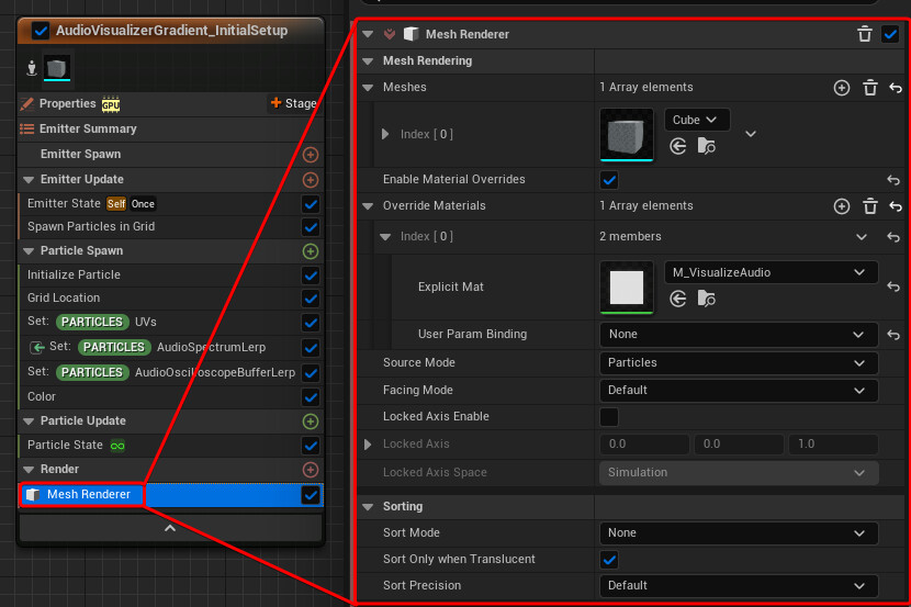
Mesh Renderer

In the Renderer I've added a Mesh Renderer and removed the Sprite one.
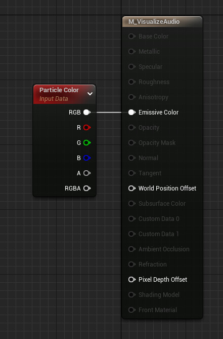
I'm just using the engine's Cube which is 1x1x1 meters and overwriting the material with M_VisualizeAudio
M_VisualizeAudio is just an unlit Material that uses The Particle Colour as Emissive.

---

Sample Audio

Now the Emitter is ready to go and we can start working on the Sample Audio Module.
The module is added to the Emitter in the Particle Update section and has a Map Get node with the following inputs:

  • New Audio Spectrum → Audio Spectrum → uses the matching User Parameter shown previously in the post
  • New Audio Oscilloscope → Audio Oscilloscope → uses the matching User Parameter shown previously in the post
  • UVs → vector2D → uses the particle's UV Attribute shown previously in the post
  • Sensitivity → float → could also be exposed as a User Parameter

Both the Audio Spectrum and Audio Oscilloscope get sampled using the Audio Spectrum and Sample Audio Buffer nodes respectively which are also using the U value of the particles' UVs Attribute for sampling.
Then they get multiplied with the Sensitivity float input to change their intensity, I'm also multiplying the Audio Oscilloscope by an extra value of 10 because I noticed that its result is generally smaller compared with the Audio Spectrum's.
Then I'm clamping the values between 0 and 1 with Saturate nodes and set them as new Particles Attributes
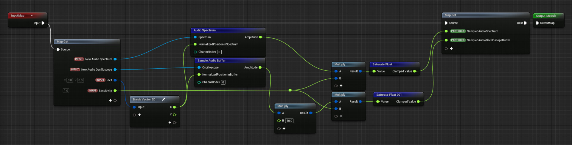
Looking back I think I would have added the switch logic here, so that the module only sets one attribute and based on a Boolean it switches from using the Audio Spectrum and Oscilloscope. This is especially useful if you need to reference the sampled audio attribute in multiple modules in the FX.

---

Sampled Value Uses Examples

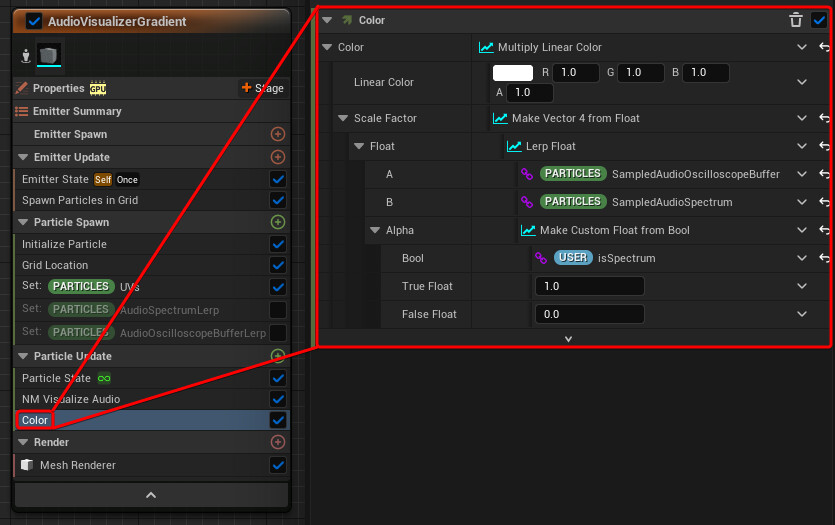
Now you can use the sampled audio value as a lerp to animate the particles in various ways, a very simple example is to just change their colour.
Below you can see how it can be used in a Color module to animate their brightness, in this case I've done it with a multiply operation but you can lerp between 2 distinctive colours as well with a lerp. The logic also includes if it should be using the Audio Spectrum or Oscilloscope sampled value.
Result:

For my Equalizer Classic FX I've used the sampled audio value to scale and offset particles as well.

---

Fade Sampled Audio

A technique I found useful is to fade out the sampled value over time so that it slowly reaches 0 instead of being hard set to it when there is no sound playing.
I've duplicated the emitter and moved the particles down from the Grid Location module, so that I can compare the 2 results.

The module takes the Sampled Audio and Lerp attributes for both the Audio Spectrum and Oscilloscope. These could actually be hard referenced within the module, but in this case I've exposed them as inputs and manually input them in the Module's Emitter.
The module also takes the User Parameter FadeSpeed.


The logic looks a little bit convoluted but what it's doing is comparing the Sampled audio value with the Lerp one.
If the sampled audio is bigger the lerp value it gets hard set to it, so that they match.
Otherwise a small float amount (FadeSpeed) chips away from it with a subtraction operation, so that it slowly reaches 0 and when it does the value keeps getting set to 0 until a new sound is heard.
On the right the same logic is duplicated, but applied to the Oscilloscope attributes.

Result:

If you know a better way to achieve this please let me know!

---

Sample from Custom Submix

At the moment when the Niagara System is placed in the level, I've always used the MasterSubmixDefault as the input for the Audio Oscilloscope and Spectrum sampler, which is what every tutorial online tells you to use.
The problem I had with this is that every sound that is played in the level is sent to the MasterSubmixDefault, which means you can't use it when you have multiple sounds playing in the level and you want the FX to react to only specific cues.
I've never really used audio much in Unreal so this was all new for me, I wanted to share my findings because I noticed there isn't much information online.

To achieve this you need to set up your own Submixes, for testing purposes I created 3 of them:

  • MasterSubmix → my new custom Master Submix
  • BackgroundSubmix → Submix that will contain background noise sounds
  • MusicSubmix → the Submix that will contain the Music I want my FX to react to

I've then connected them as follows inside the MasterSubmix

One important thing to do is to change the Project's default Master Submix in the Project Settings

Now we need to tell the various Cue assets to which Submix they should be sent to. This can be done by creating Classes Actors that then get applied to the Sound Cue Assets.
Same as the Submixes, I made 3 of them:

  • SC_Master
  • SC_Background
  • SC_Music

I've connected them as follows but I noticed that it doesn't really matter, so I'm not sure what this actually does (let me know if you do!)

However what you do need to do is to change their Default Submix to the matching one for both SC_Background and SC_Music

Now you can open up the Sound Cue Assets and set their Class based on what Submix you want to send them to.

I think this is the approach you would want to follow when working on a big project, having Sound Classes feels like the way to go to better manage sound.
However, I found you can actually set the Submix directly in each Sound Cue asset avoiding having to set up Sound Classes, if this parameter is set then the value overwrites the Class' settings.

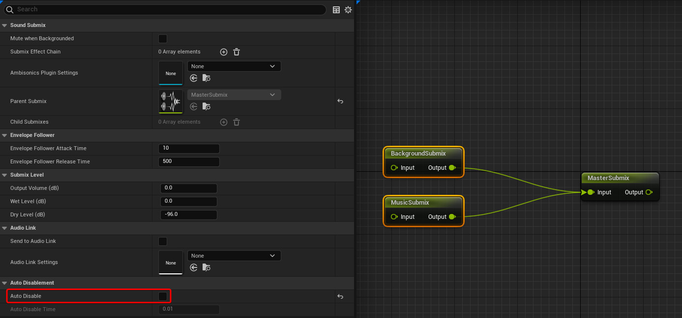
The main issue I've encountered doing this is that when everything was setup when I was feeding my custom Submix to the Niagara FX the particles wouldn't react at all.
I posted on Unreal's Forum about it and I have to thank @James.Wizard for replying with a solution.

Turns out the Submixes have the option to get automatically disabled when they are silent as a CPU optimization, the problem is that they should get re-enabled if the sound is sent to them, but it doesn't look like that's happening because by turning off the feature the Niagara FX starts reacting as expected (this project was done using UE5.1.1)

In the video below there are 3 Niagara systems, and each of them is assigned to a different Submix

---

Conclusion

I hope you found this tutorial useful, if you do create an FX that is driven by audio please share it with me I would love to see it!
Thanks for reading and have a great rest of the day!


Report

Create Content Plugin - Unreal Engine

Tutorial / 16 February 2023


Introduction

Sometimes when working on a project you might be creating something useful that you want to use again in the future, creating a Content Plugin is an easy and clean way to do that, an alternative to just migrating the assets from project to project.

This is a very simple step-by-step guide aimed at beginners.


Plugin Creation

The plugin can be created from the Plugins Window, to open it go to Edit → Plugins


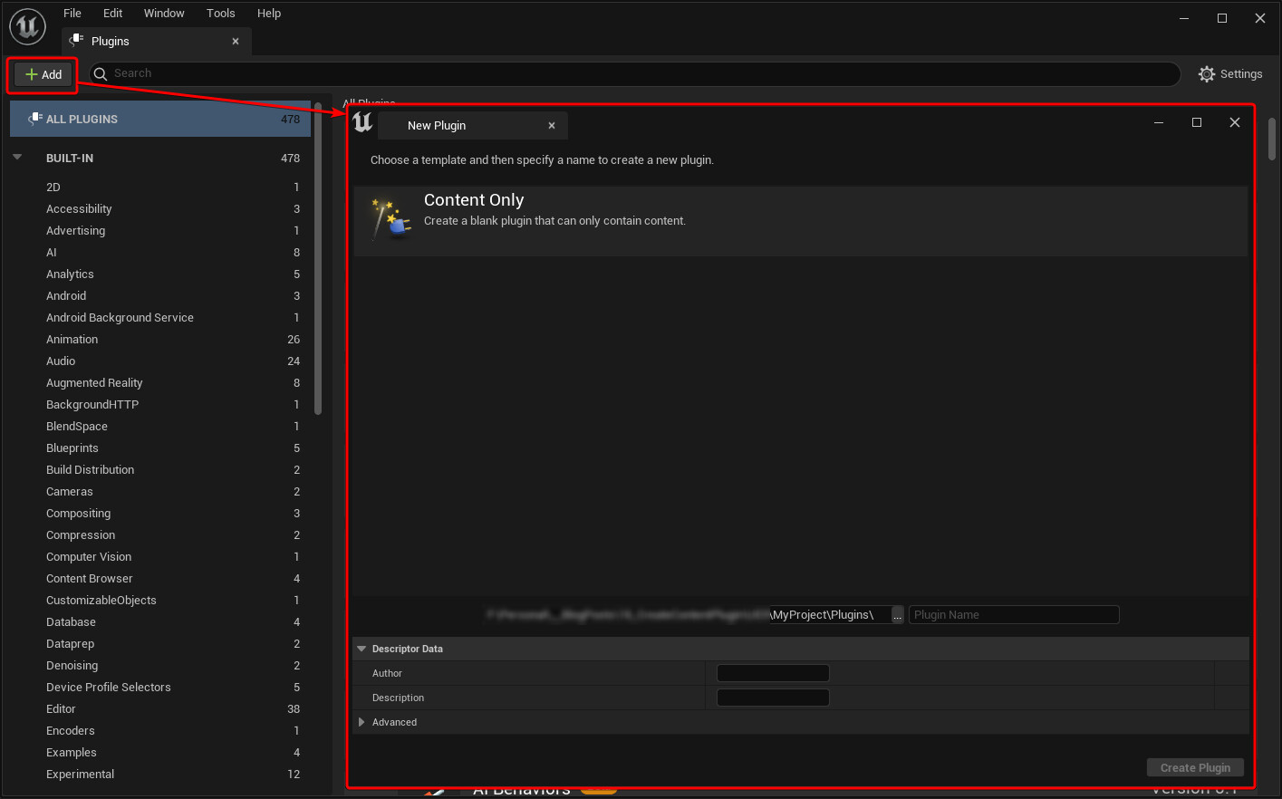
Now press on the Add button, which should open another pop-up window called "New Plugin"


From here you can create the plugin, click on "Content Only", then add a name, fill up the descriptions prompts, and press the "Create Plugin" in the bottom right.


This should make the folder "Plugins" appear if it wasn't there already, and a new folder called "YourPluginName Content" gets created.
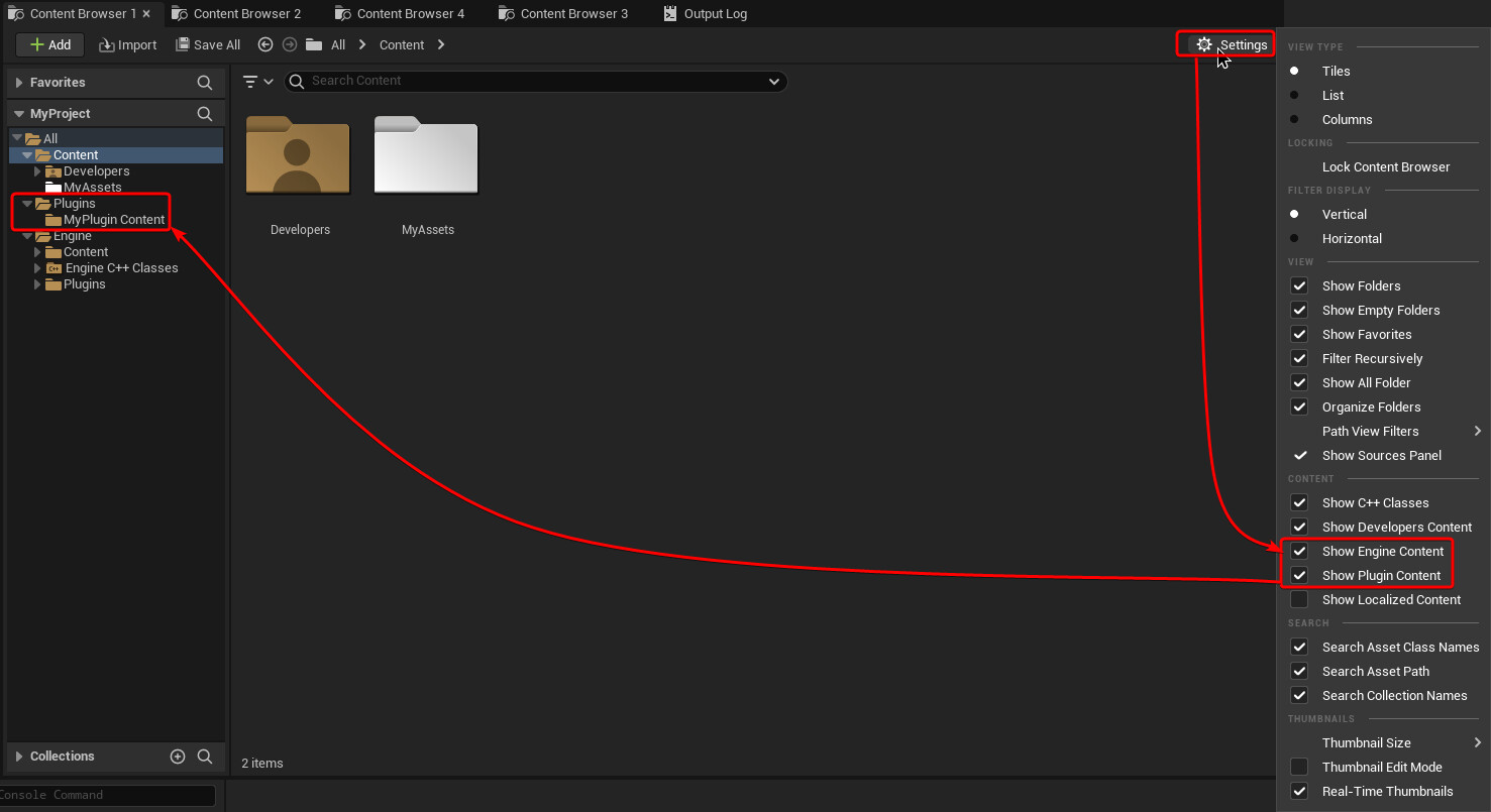
If you don't see them make sure you have both "Show Engine Content" and "Show Plugin Content" on, you can check them by clicking under "Settings" on the top right of the "Content Browser".


Now that it's created you will be able to see it in the "Plugins" windows, under the "Other" tab.


Pressing the Edit button a pop-up window appears where you can change the Plugin's Icon, Details and even add Dependency plugins to it so that once it's activated Unreal prompts you to activate other plugins that need to be on for it to work. A good example is if your plugin contains HDAs, Houdini Engine Plugin can be added as a dependency.


Populate the Plugin

In the project, I have a folder called MyAssets which contains everything I want to include in my Content Plugin


To populate the plugin with this content you can just move all the files into it


And just in case, I would Fixup Redirectors to prevent references issues


Moving Plugin to Another Project

Once you added content to the plugin you can keep working on it, editing, adding, and removing things.
When it's completed and you want to reuse it in another project you can package it by finding it in the Plugins Windows

After selecting the saving directory and a couple of pretty and futuristic compiling and competition sounds, a new folder with the name of your plugin will be created, that contains all the uasset.
Move it to the new project's directory, in the "Plugins" folder, following the same folder structure it was in the original project:

MyProject → Plugins → MyPlugin


If you open now the project the plugin will be already installed and activated automatically, if it had dependencies Unreal will ask you to activate the respective plugins and then probably restart.
If you don't see it make sure again both "Show Engine Content" and "Show Plugin Content" are turned on.


Conclusion

I hope you find this post a useful resource to get introduced to plugins and that you'll use this approach when reusing content for future projects!
Have a great rest of the day!

Report

Houdini - Switch When Input is Empty

Tutorial / 08 December 2022


Introduction

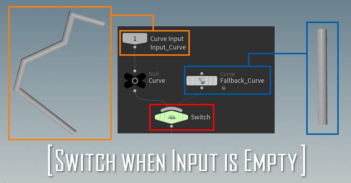
This post will show various ways you can use a switch node to automatically trigger when one input is empty, a very useful technique when working with HDAs.
Especially important when working with complex generators, this way you can still get a preview of your output, or even prevent the node to fail cooking or getting stuck in infinite loops when using the HDA in Unreal Engine.


Setup

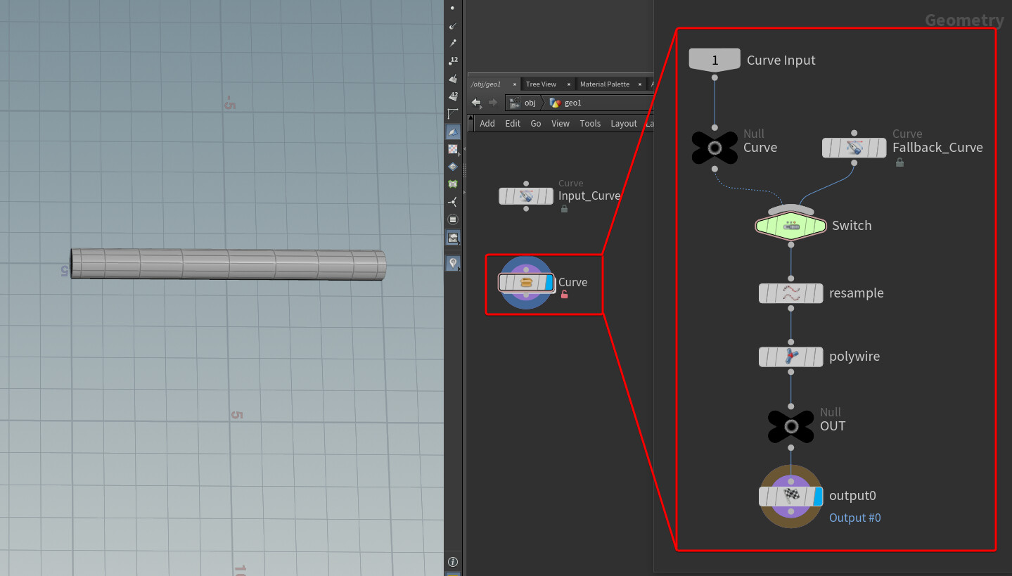
For showing off the technique, I prepared a simple setup with an HDA that applies a Polywire operation on the input curve

The HDA graph:


Switch node

You can see the Switch node has 2 inputs, one is the input curve and the other one is another curve used as a fallback option.
The easiest way to make the switch activate and use the second input is to check the number of points of the first one, if they are equal to we can trigger the switch.
For more complex cases you might want to check if the points are less than a certain value, in this case since I'm working with a curve I want the input to have at least more than 2 points, and use the fallback option for anything less than that.
This can be done with a simple expression:

if (npoints("../Curve") < 2, 1, 0)


The "if" function takes in 3 floats, in the first one we can input the check expression we need to do, while the second one is the output value if the expression is true and the third one when it's false.

if(<expression>, <true_value>, <false_value>)


Now, if I remove the input to the HDA or if I feed to it something that contains only 1 point it will use the Fallback Curve which in my case it's a simple straight line.


Simplify

We can actually simplify it further, at the moment the input for the "npoints" function is a hard reference to one of the nodes in the graph, but we can simply replace it with "0" since the node we want to check is one of the inputs. The same way you would do when using a Wrangle Node.
So the below expression will give us the same result:

if (npoints(0) < 2, 1, 0)


Trigger from Other Nodes

If you do need to drive the switch using another node you can do it using the first example shown, having the name hard coded:

if (npoints("../Check") < 2, 1, 0)

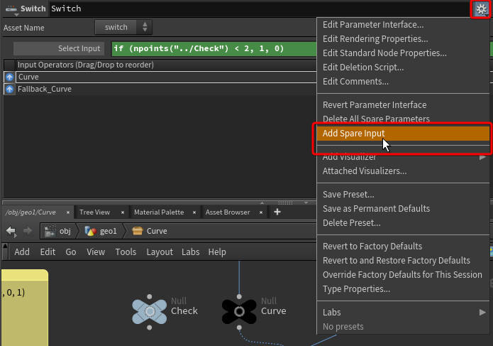
But better than that, to make it more clearly visible for anyone looking at your graph or for your future self when coming back to it, you can use a Spare Input.
Create by clicking on the cog icon:

Now if you click and drag your Check node in the Spare Input Slot you will create a reference and now you can use "-1" in the expression to access it.

if (npoints(-1) < 2, 1, 0)


Switch-If node

This node only takes in 2 inputs but it gives a lot of options and operations to trigger the switch, like checking if attributes or groups are present or equal to specific values.
I haven't played much with it myself with these options, but the same expressions shown above work with this node as well.


Here I found you could even just use "npoints(1)" and switch the order of the inputs, because everything above 1 gets clamped.
So if there are no points in input 1, the result of the expression will be 0 and the first input will be used instead.


Conclusions

I hope you found this post useful for your future HDAs, have a great rest of the day!

Report

2D SDF - Gradient/Flowmap and AA technique - Material Function Library UE5

Tutorial / 04 October 2022


Introduction

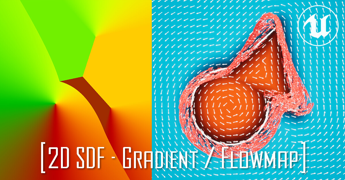
In this post, I'll show you how you can create a gradient from a 2D SDF and how it can be used as a flowmap in the material to warp a texture or in Niagara to drive the location of particles! I've also added a bonus section about Anti Aliasing, something that I haven't covered before.
If you haven't seen my previous posts about SDF I highly recommend them:

  1. Basic Shapes and Visualization
  2. Combine Shapes
  3. Manipulate Space


Gradient / Flowmap

Shape

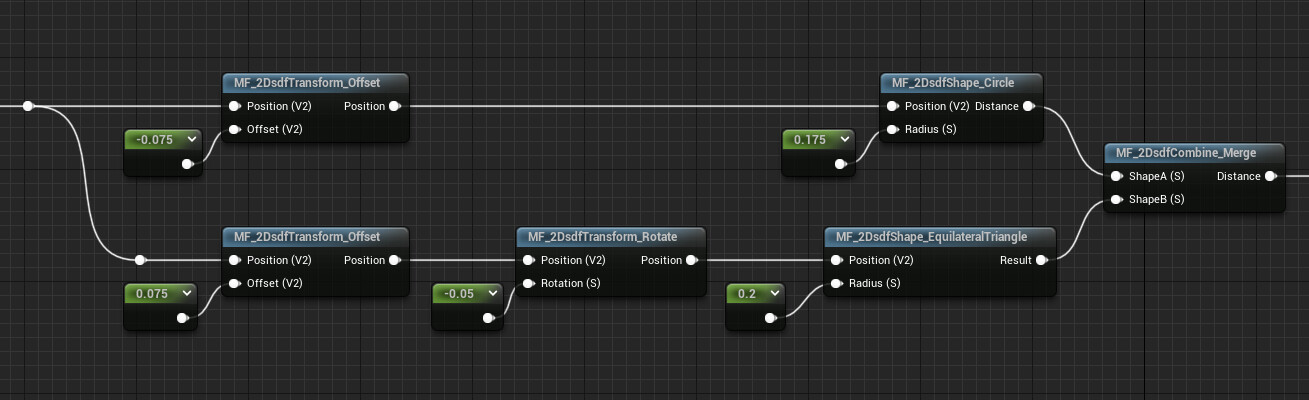
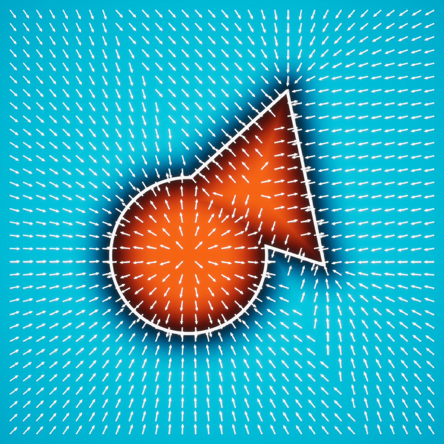
For the rest of the post I will use an SDF of a sphere and a triangle combined together that looks like this:

Here's the graph, you can find how to create these functions in my previous posts:


Explanation

For understanding how to make gradients form SDFs I've read this post, have a look at it if you want some more in detail explanation.

If you've read my first post about SDFs it's probably you should know that each point in the field of an SDF stores the distance to the closest edge of the shape, we can use this information to calculate a gradient, which will be a direction that points either directly towards or away from the closest edge. This is done by comparing the value of each point in the field to the value of their neighbors on the X and on the Y axes.

The arrows in the image above show the gradient.
Inside the field, where the distance is negative, the gradient points directly towards the edge.
Outside it, the gradient points directly away from the edge.
These directions can be expressed as a 2D vector, which is referred to as the gradient vector.


Logic

The only thing to keep in mind is that this gradient doesn't come cheap, to generate it we need to sample the sdf two extra times, with some offset on the X and on the Y to calculate the derivatives of the two axes. This just means that we need the change of rate in both X and Y.

Because we need to sample the SDF three times I would highly recommend creating a Function that contains the shapes of the SDF you are working on, especially if you're manipulating and combining multiple shapes.

We first need to sample the distance as usual, then to calculate the change of rate in the X axis we need to add a slight offset on the position and then sample the SDF again, this way we are essentially finding the Right Neighbour value for each point in the SDF. Then subtracting it from the distance calculated earlier, we get the change of rate on X. We can do the same for getting the Top Neighbour of the SDF and the change of rate in Y.
If we then make a Vector2 appending the two results and normalize it, we get the gradient.

And here it is in all its glory:


Warp Texture

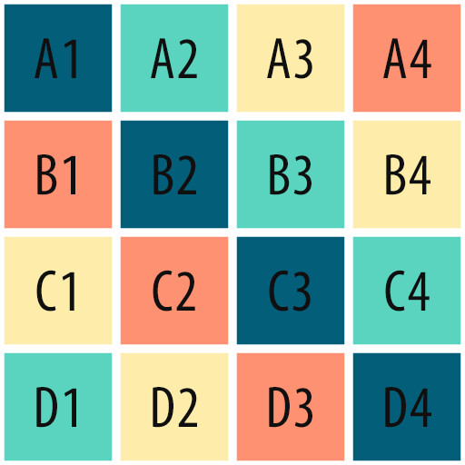
This gradient can be used as a flow map to warp and distort textures, for my examples I will be using this texture with some tiling:

For demonstration purposes, I've only set up a simple example.
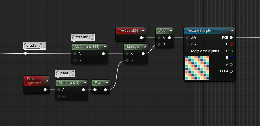
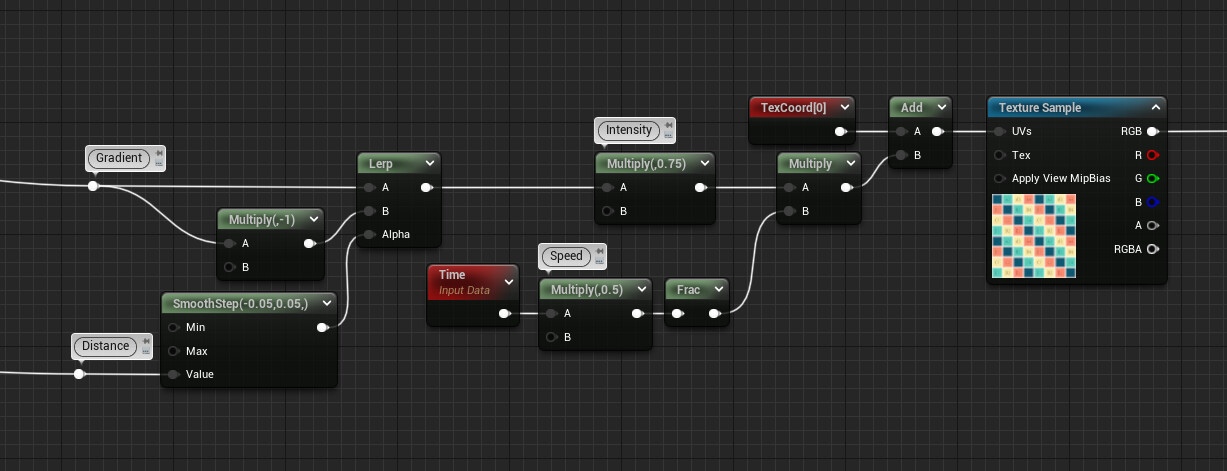
You can multiply the gradient to control the strength of the warp, then multiply again with Time and add it to the UVs of your texture. I'm also controlling the speed multiplying Time and I'm feeding it to a Frac node to have the distortion happen in a repeating loop:

You can see that the texture will move outward from the center of the SDF, just like the direction of the arrows shown earlier:


Of course, we can mask this distortion using the distance value of the SDF, in the example below I'm inverting the direction of the flow for everything that is outside of the shape and keeping it the same as before for the inside. This can be easily done with a Lerp node, in this case, I'm also using a Smooth Step function to remap the SDF (again, more about this in my previous posts)


Render Target

What's cool is that we can draw both the distance and the gradient of the SDF to a Render Target and read the texture in Niagara to control the location and low of particles!!

When drawing the Material to a Render Target we need to keep in mind that we can only have values in the range of 0 to 1. However, we know that the distance of the SDF contains negative values for the points inside the shape and the directions of the gradient also contain some negative values. So we need to lift them all to be in the range needed, this can simply be done by adding 1 and multiplying by 0.5.

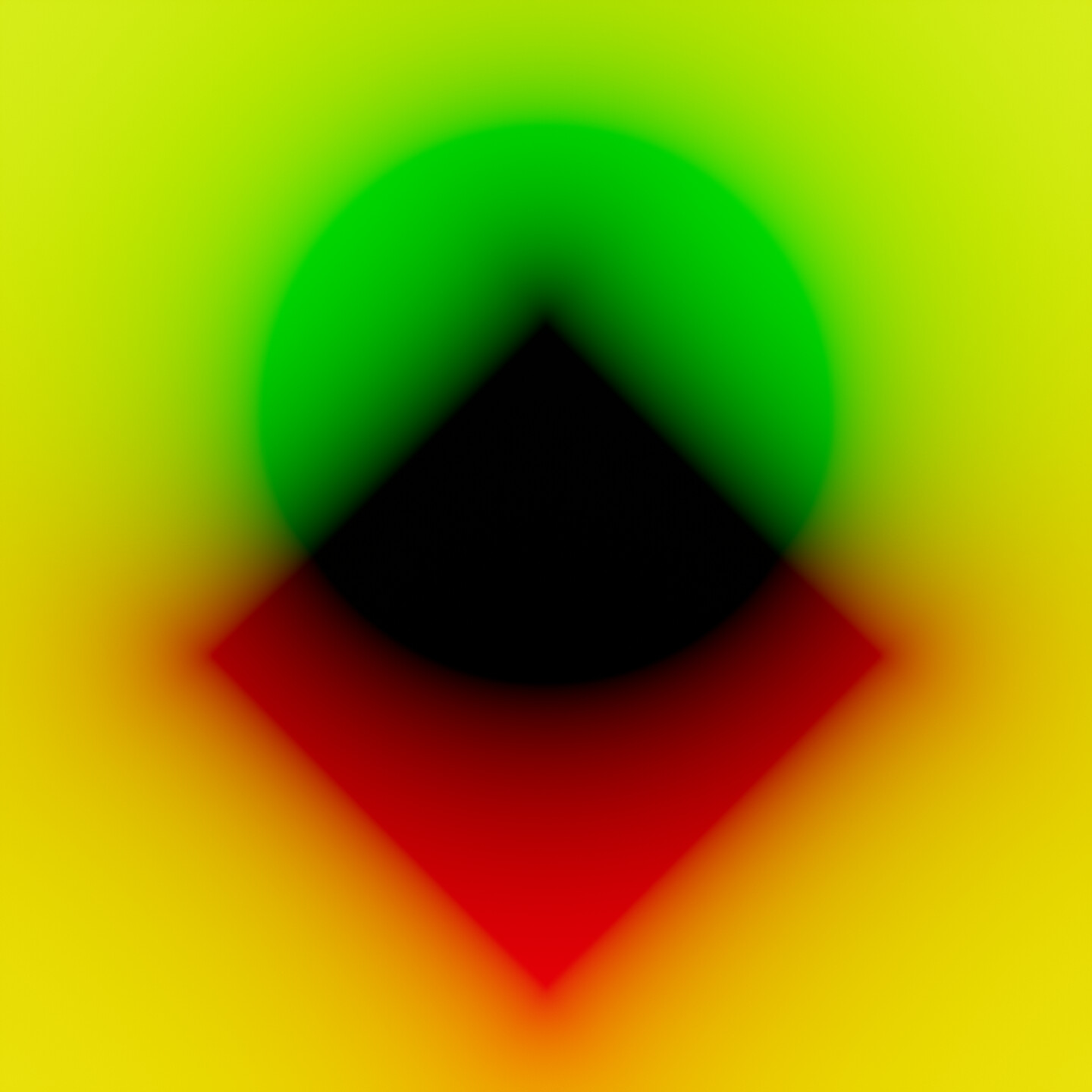
What I also like to do is to combine them both in a vector3, having the distance in the Red Channel and the gradient in the Green and Blue ones.

This is what it will look like:


Niagara

In Niagara you can use the built-in Sample Texture module, here you can feed your texture directly or have it as a user parameter, the only other thing needed is some UVs!
If you're spawning the particles with the combination of "Spawn Particles in Grid" and "Grid Location" modules, you can use the attribute GridUVW that gets created. Otherwise, if you're simply using a Shape Location module set to Box/Plane, like I'm doing, we need to make the UVs based on their position.

To do that I made a vector2D particle attribute called "UVs" and I'm setting it using the Scratch Dynamic Input. Below you can find the graph, I'm getting the position and dividing by the size of my plane (which is 100 in my case), then I'm making the Vector2D getting only the 2 axes I'm interested in and adding 0.5 to offset the origin from being in the center of the plane to a corner in the bottom.
Note that to make this setup work you need to have the Emitter be in Local Space, if that's not possible you need to take into account the World Position of the Actor in the level and offset the particle position value accordingly (I believe you can do it by using the Engine Emitter Attribute "SimulationPosition", but I'm not 100% sure).

Of course, if you need this setup in multiple Niagara Systems I suggest creating an actual Dynamic Input asset for it, with the size of the plane exposed as a parameter.

I might write something more in detail about this topic in a future post, for now, let's get back to our SDF.

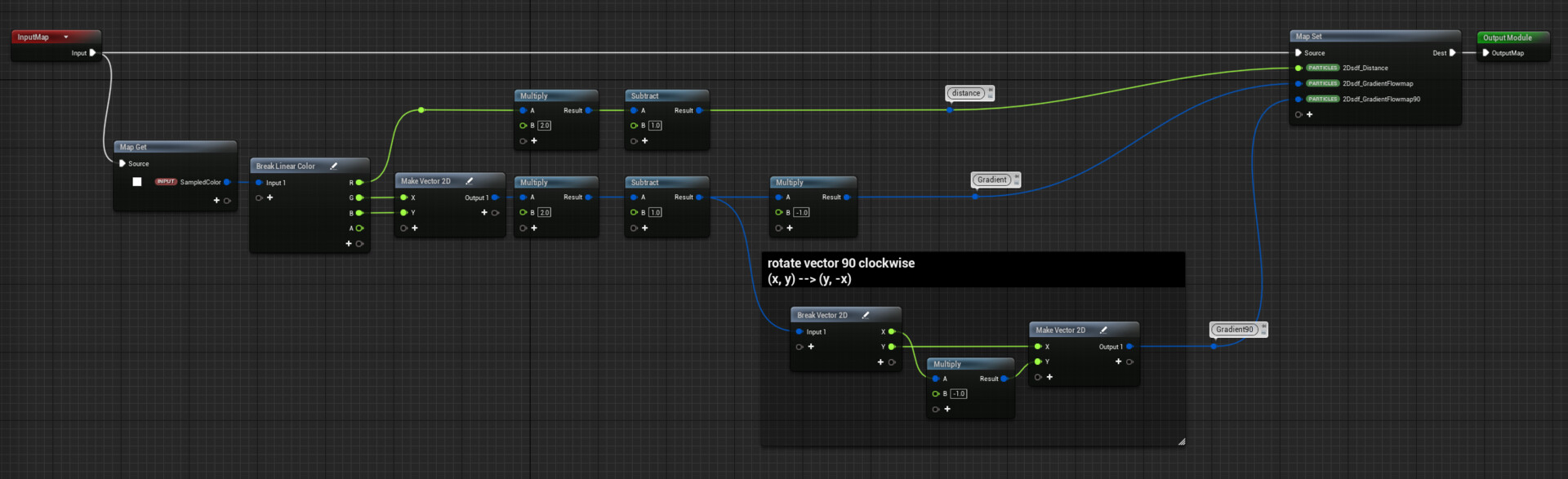
Now that we sorted out the UVs we can sample the texture with the Sample Texture module mentioned earlier, this module creates a particle attribute called SampledColor that contains the values of our packed texture. We can use a custom module to unpack it and remap these values back to -1 to 1 and create particle attributes for both the distance and the gradient.
This can be done by multiplying by 2 and subtracting 1, then since I want to make particles flow around the SDF shape I've rotated the gradient by 90 degrees and saved it as another attribute.
To rotate a 2D vector by 90 degrees you can invert the order of x and y and multiply x by -1:

(x, y) --> (y, -x)

If we visualize the vectors of the rotated gradient they look like this:

Now if we align the direction of our particles using the gradient vector as is, we'll get the result I showed during the explanation part of this post. What we can do is use the distance information as well to invert the direction base on if the particles are inside or outside the SDF shape:

We can use these vectors to attract the particles towards the shape's edge, multiplying it by a force and adding it to the Transient Attribute PhysicsForce so that it gets applied to the velocity in the Solve Forces and Velocity module. We can do the same for the rotated gradient.

That's the main logic needed to have particles move along the SDF edge:


The power of this setup is that if we can have the texture baked out if the SDF doesn't move, but if it's animated we can feed the RT directly and calculate the new SDF distance and gradient in real-time getting some very cool results like this one:


Anti Aliasing

Introduction

When working with these shapes and you're using a Step function to visualize them, you might have noticed some aliasing or flickering around the edges, it's not much since we are working with procedural shapes instead of using textures but in some cases, it might be more evident. Fortunately, there is an easy solution!

I did some research online on the topic and I would recommend you to read these 3 sources:

  1. numb3r23 - Using fwidth for distance based anti-aliasing - the technique I used and will explain below 
  2. mortoray - Antialiasing with a signed distance field - interesting read, but the SDFs, in this case, need to be calculated in pixels
  3. drewcassidy - Antialiasing for SDF textures - might be useful if you're working with SDF textures

Function

We can introduce some anti-aliasing using the Smooth Step function, we want the interpolation to only happen on the edge of the SDF shape, basically the size of one pixel. To achieve this we need to calculate the "anti-aliasing-factor", which will basically tell us the rate of change in the distance field.
This can be calculated by feeding the distance of the SDF directly in the fwidth function: 

float aaf = fwidth(dst);

Unreal's Material Graph doesn't have a node for that, but fwidth is simply the sum of the absolute values of ddx and ddy - check out this video to learn more about these three functions.

dx = ddx(v);

dy = ddy(v);

fwidth(abs(dx) + abs(dy));

Now, the size of the rate of change in the distance field given us by the "anti-aliasing-factor", determines how wide the Smooth Step interpolation needs to be in order to fade the edge of the SDF shape:

return 1.0 - smoothstep(radius - aaf, radius, dst)

I would replace the step function with this one almost in every scenario, it's very useful when using the SDF as the opacity for a masked material or the alpha when lerping between two colours.


Conclusion

For now, this is everything I wanted to share about 2D SDF, in the future I would like to experiment more with 3D SDFs to create some interesting FXs with Niagara.
I hope you found this post insightful, have a good rest of the day!


Report

2D SDF - Manipulate Space - Material Function Library UE5

Tutorial / 15 September 2022


Introduction

This is the third part of a series of posts about 2D SDF, check out the first one where I show some simple shapes and explain the basics to visualize them, and the second one where I show different ways to combine them!
I think it's very useful and valuable knowledge for every Technical or Environment Artist, but really for anyone that works with materials.
In this post, I will cover ways to manipulate the space used to sample these shapes, as well as share some extra tips I've learned along the way.
As I mentioned before, everything I will cover is not new knowledge, I've learned it all by reading Ronja and Inigo Quilez's articles which I highly recommend for getting a better understanding.
The focus of my posts is to show how their content can be recreated in Unreal Engine and its Material Graph.

I'm sorry again if this is another long post, but I hope it's worth reading, enjoy!!


Distortion

I found a couple of ways to add some distortion to the perimeter of the shapes.
The first one involves sine waves, while the second one 2D or 3D noises. The only thing to flag is that doing this will make the distances of the sdf functions less precise, but if the intensity and the amount of these distortions are low, in most cases this is not a problem.
For all the direction examples shown below, I'm going to use a simple square shape.

Wobble


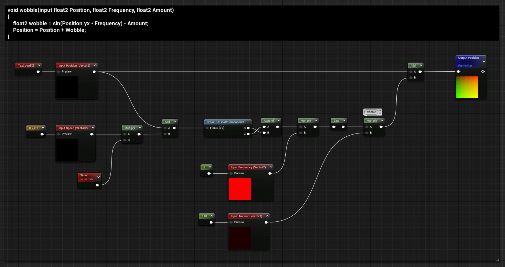
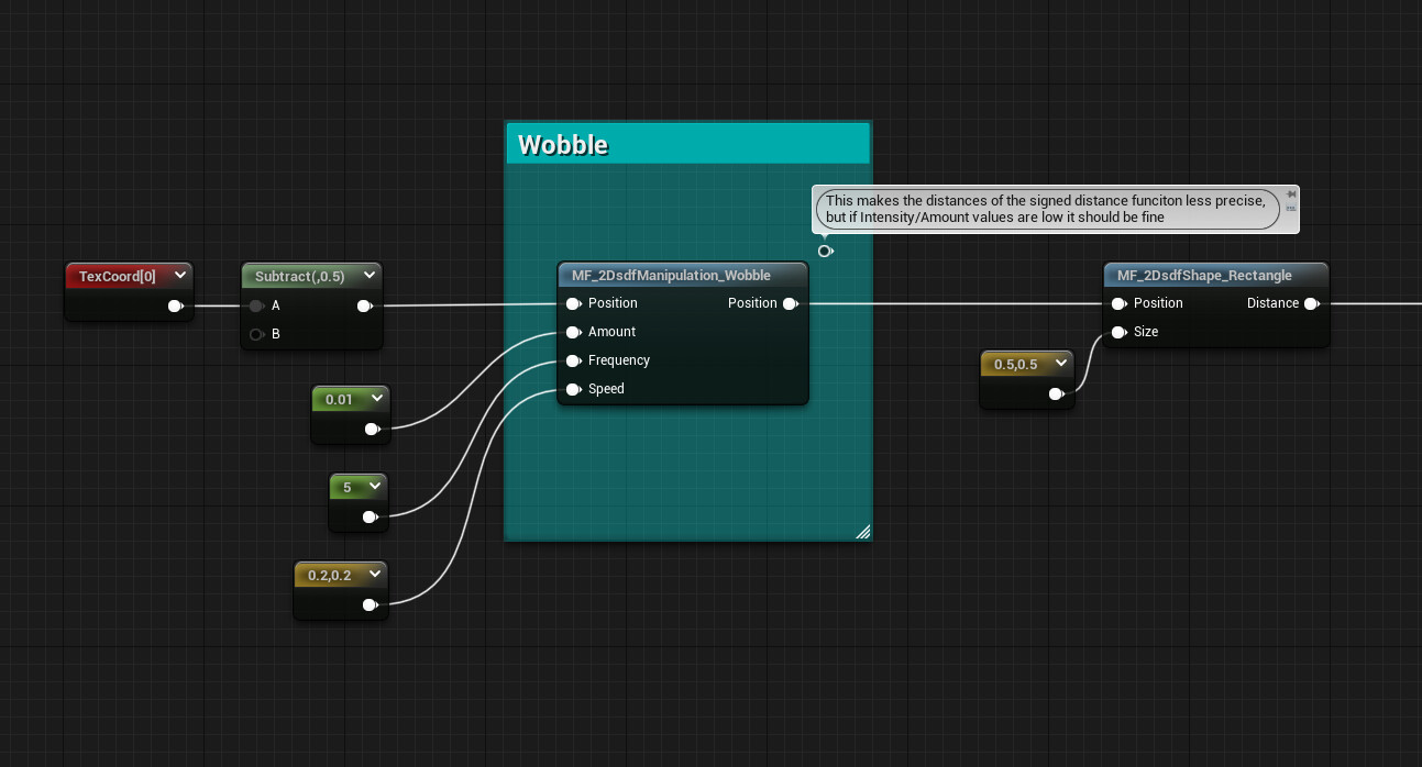
Distortion can be added using sine waves, we can do this by calculating two different sine waves, one for each axis, and adding it to the position used to sample the sdf shape. All the inputs expect a vector2, this is so that you can have separate control on the two axes.
To calculate the wobble we need to flip the x and y components, then it can be multiplied to control the frequency, feed the result to a sine node and multiply it again to control the intensity. The distortion can be animated by adding time before flipping the position, and the speed can be controlled with another multiplication.

void wobble(input float2 Position, float2 Frequency, float2 Amount)
{
    float2 wobble = sin(Position.yx * Frequency) * Amount;
    Position = Position + Wobble;
}

Multiple wobble functions can be added together to get more variation and a more complex result


Noise

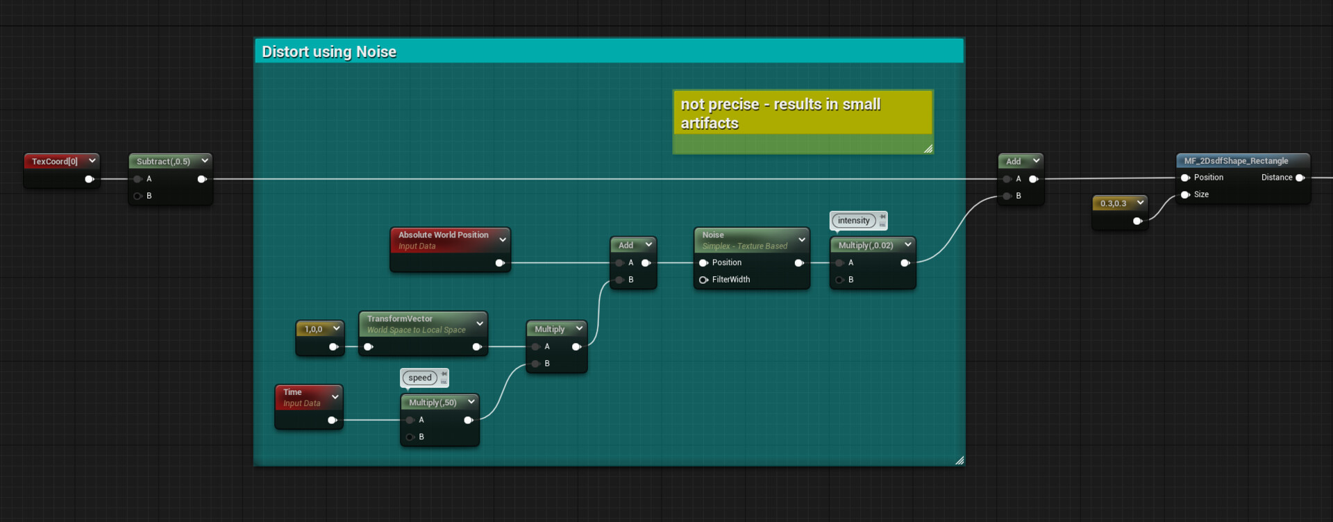
For the noise, the logic it's the same, do some multiplications to control its intensity and speed and then add it to the position before sampling the sdf shape.
Compared to the wobble, I noticed that with this method you might get even more imprecise results and artifacts on the perimeter of the shape, so be careful with it.

You can use a 2d or 3d texture based on your options, I prefer using a 3d noise because this way I can animate it through the depth axis and easily get it to look like it's morphing.
In the example below I've used the built-in procedural noise node, I've just reduced the number of levels to 3, and its scale.
I didn't create a function for this since you might need a different one for each type of noise setup you are going for, however you should definitely make one if you're using the same setup multiple times.


Extra

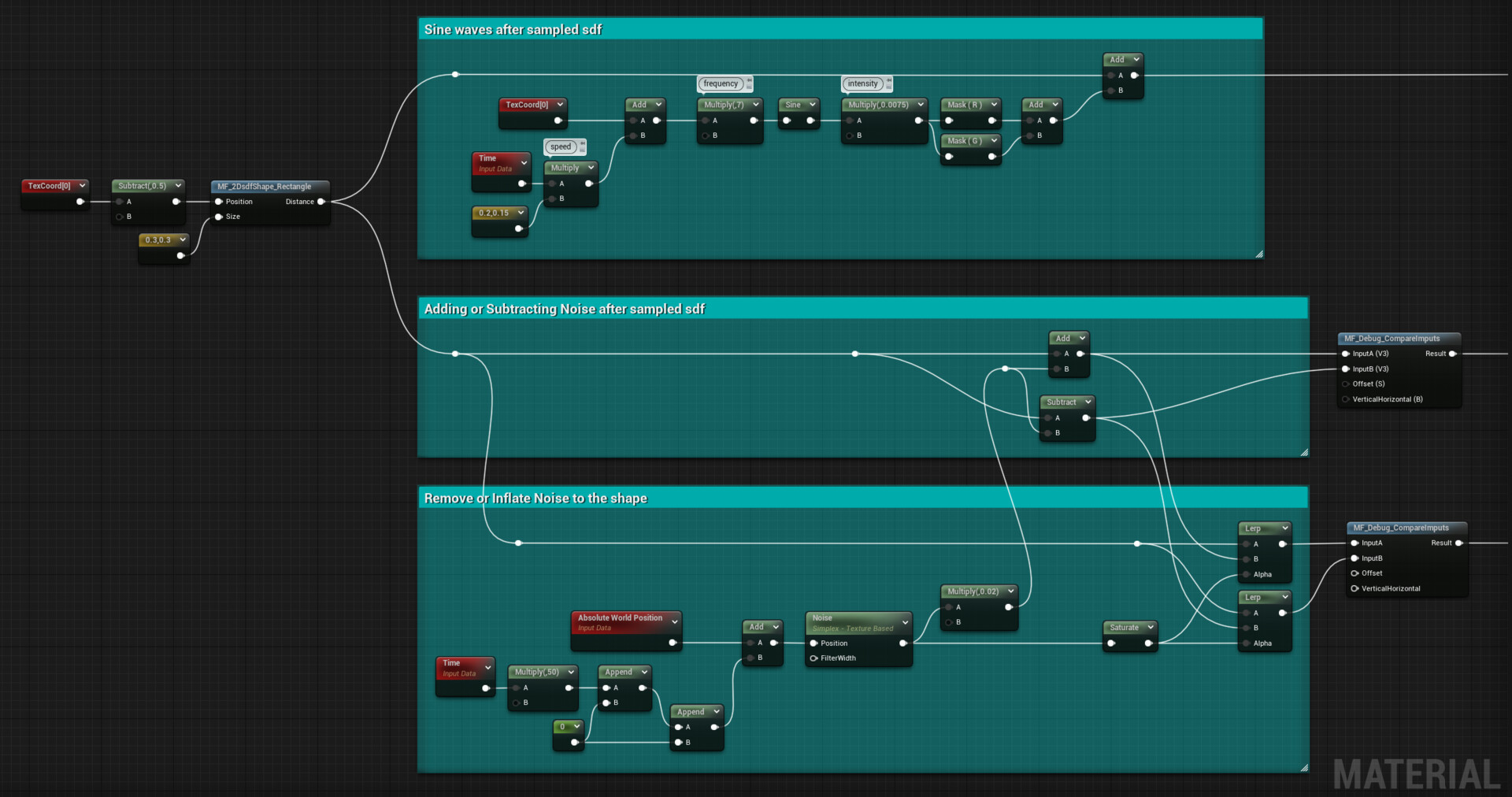
Now, I want to point out that you should definitely play around and experiment. For example, I asked myself what would happen if I did similar operations after sampling the sdf shape instead of manipulating the position.
Well, you get slightly different results of course, but is that the correct way of doing it? Who cares, if you like the result it doesn't matter. Tech Art is not always about knowing and correctly applying techniques and math, in the end, our aim is to get some beautiful results. You don't always need to understand the logic behind it, sometimes it's fun to just chuck together some nodes and values to see what comes out, you never know what you are going to get!

Below you can find some examples of some experiments, with both sine waves and noises.

Sine Waves:

Comparison of adding or subtracting noise;

Two similar setups where the noise is combined in a way so that it only removes information or inflates the shape:


Mirroring Options

Like in the way we do the shape's deformation we can manipulate the position to get some other results. Below I'll show some useful mirroring options.
Relying on manipulating the space and getting mirrored results it's a lot cheaper than sampling shapes multiple times, this way you can achieve some quite complex but cheap effects.
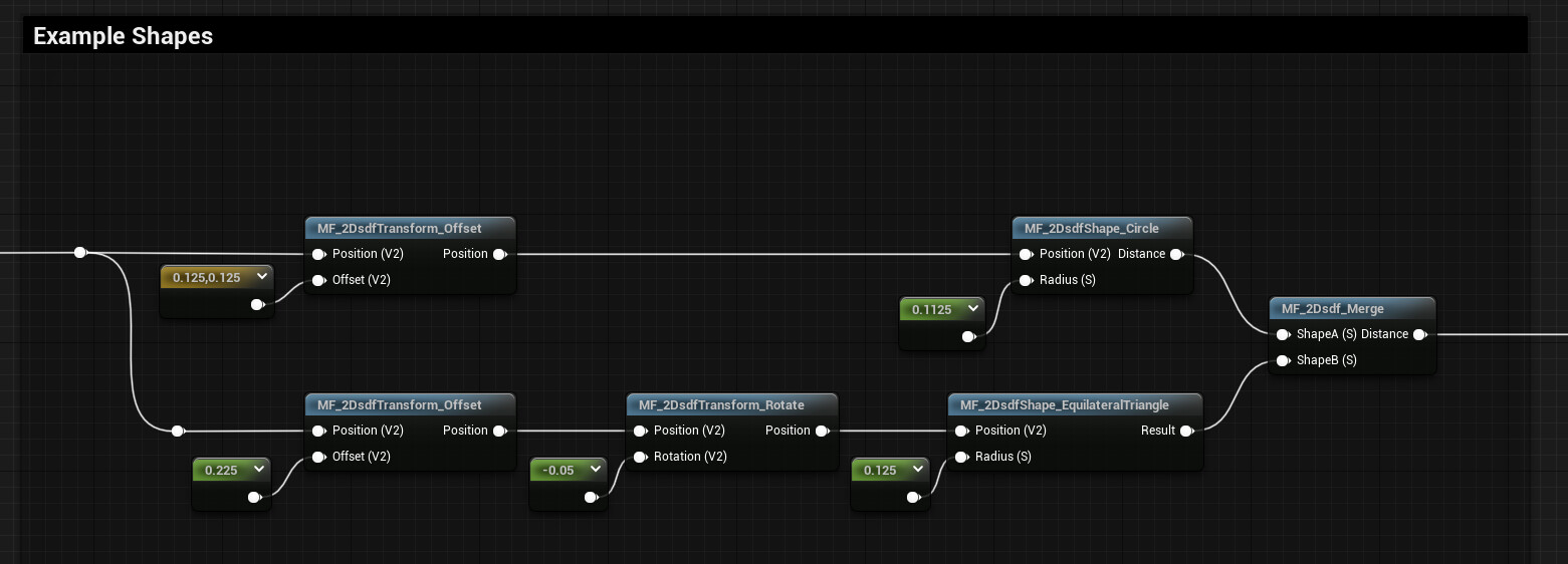
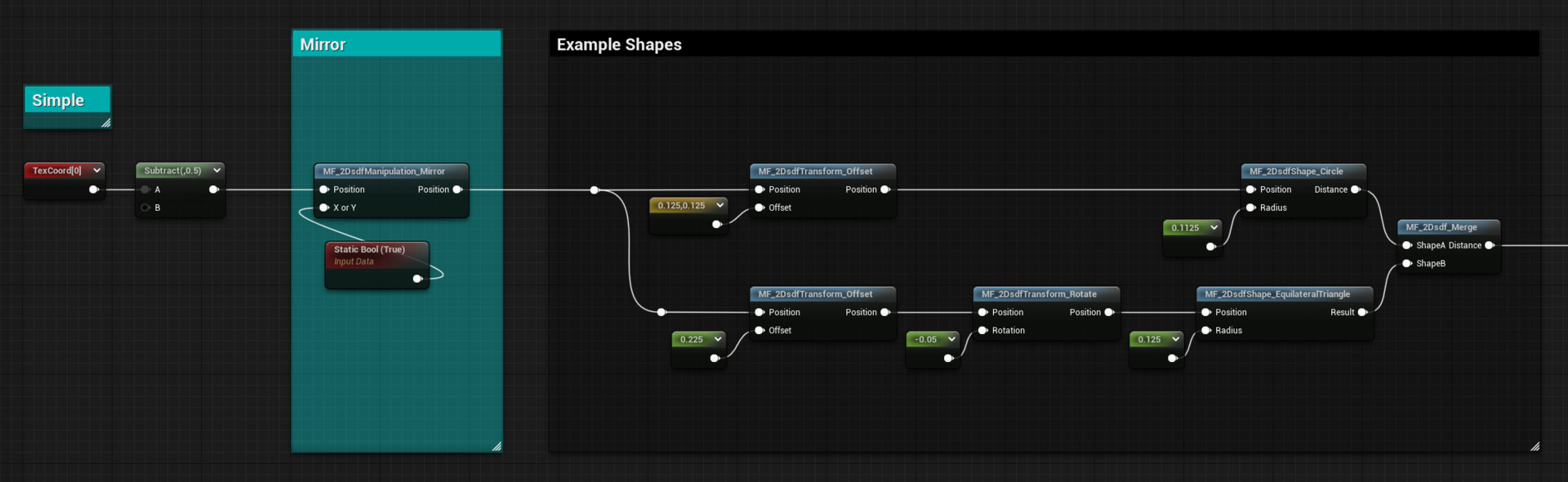
For all the mirroring options examples shown below, I'm going to use always the same sdf combination of a triangle and a circle, they both have a slight offset from the center, added using the basic transformation functions shown in the first post I made about sdfs.


Mirror

Simple Mirror


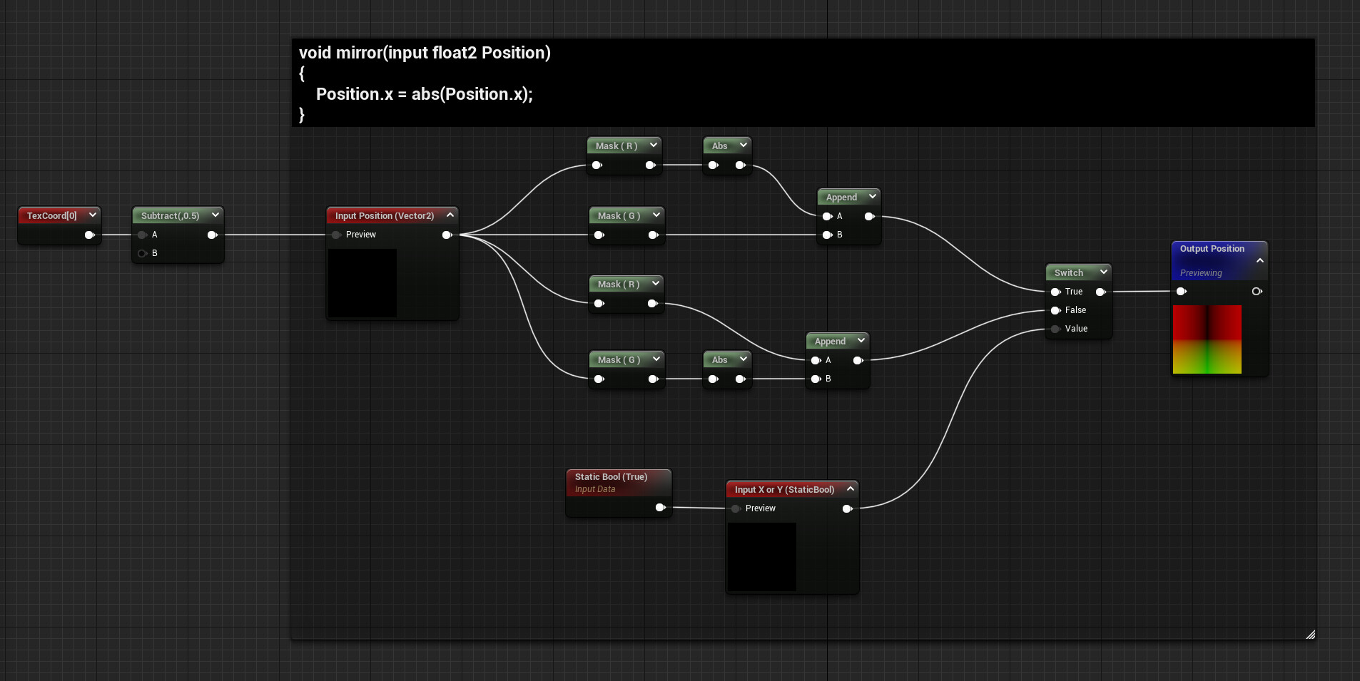
Doing a basic mirror it's very simple, we can just get the absolute values of one of the two axes:

void mirror(input float2 Position)
{
    Position.x = abs(Position.x);
}
For the function, I've also added a Static Switch to flip between mirroring on the X or on the Y axis.


Rotate Mirror

You can combine this with some basic transformation functions showcased here, I'll show you some tests with the rotation.
If you add a Rotate function before and after the Mirroring one, and you multiply by -1 the Rotation input for the second Rotate function, you can isolate the rotation to the Mirror axis:


Rotate only Shapes

Adding the Rotation function only after the Mirror one keeps the axis stationary and only rotates the position resulting in an interesting effect:


Rotate Everything

On the contrary, putting the Rotation function before the Mirror makes both the axis and shapes rotate:


Normal Cells

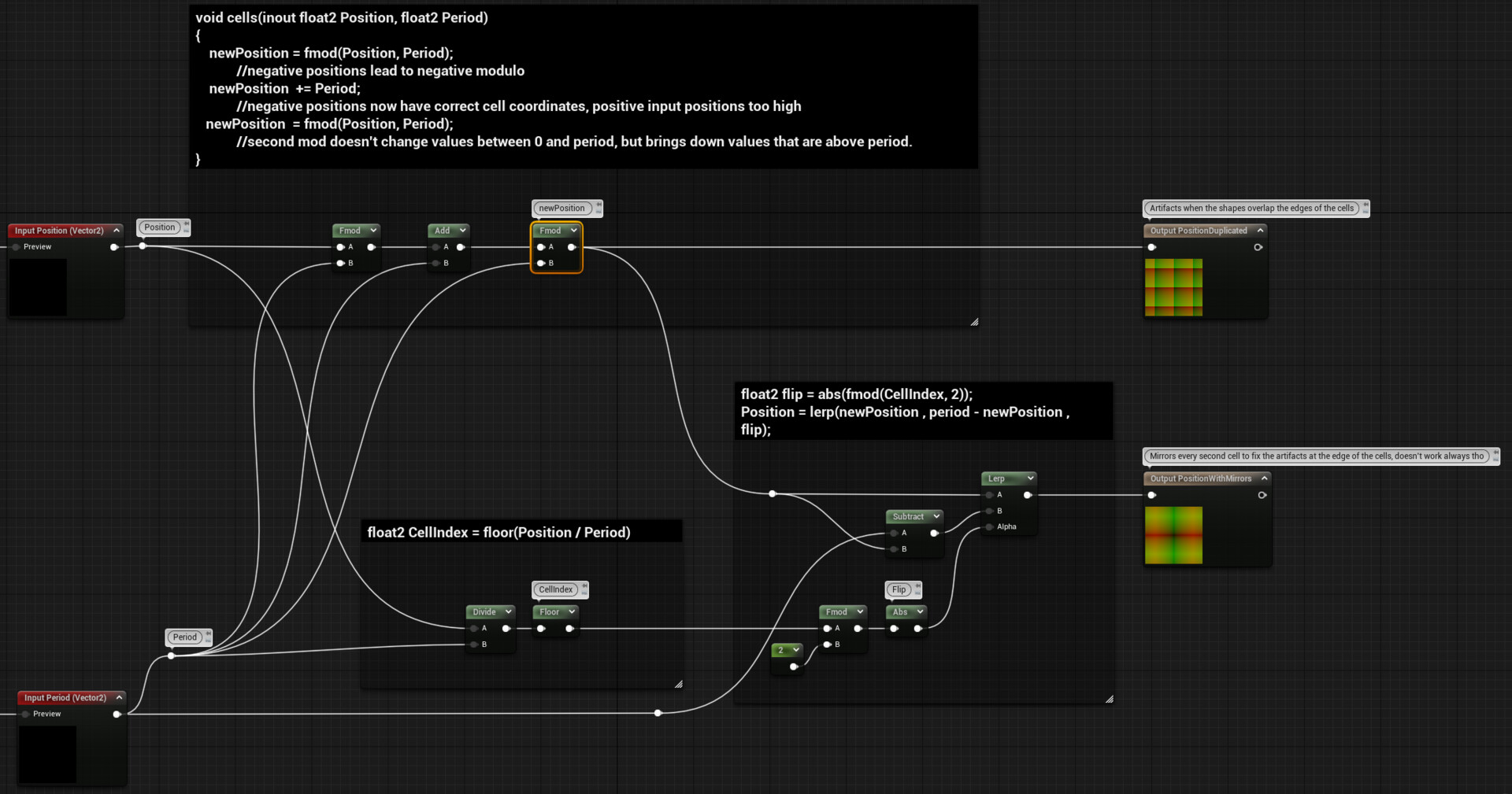
We can also tile the position in a way so that it creates cells, this function gives 2 different outputs, the first one duplicates the position like a classic tiling you can find working with textures, while the second one it's also mirroring the position.
The problem with the first output is that if the shape overlaps the edge of the cells it creates some artifacts, which doesn't happen with the mirroring option, something to keep in mind.

They both use some fmod trickery, the duplicated position function is:

void cells(inout float2 Position, float2 Period)
{
    newPosition = fmod(Position, Period);
            //negative positions lead to negative modulo
    newPosition  += Period;
            //negative positions now have correct cell coordinates, positive input positions too high
   newPosition  = fmod(Position, Period);
            //second mod doesn't change values between 0 and period, but brings down values that are above period.
}

For the Mirror output, we need to calculate the Cell Index to know which cells need to be flipped, we can add this to the previous code:

float2 CellIndex = floor(Position / Period)
float2 flip = abs(fmod(CellIndex, 2));
Position = lerp(newPosition , period - newPosition , flip);

Here's the comparison of the two outputs, duplicated position on the left and mirrored version on the right:


Radial Cells

This one is a little bit more complex, as it always is when rotations are involved, as I mentioned before check out Ronja's tutorial for a more in-depth explanation of how this works.
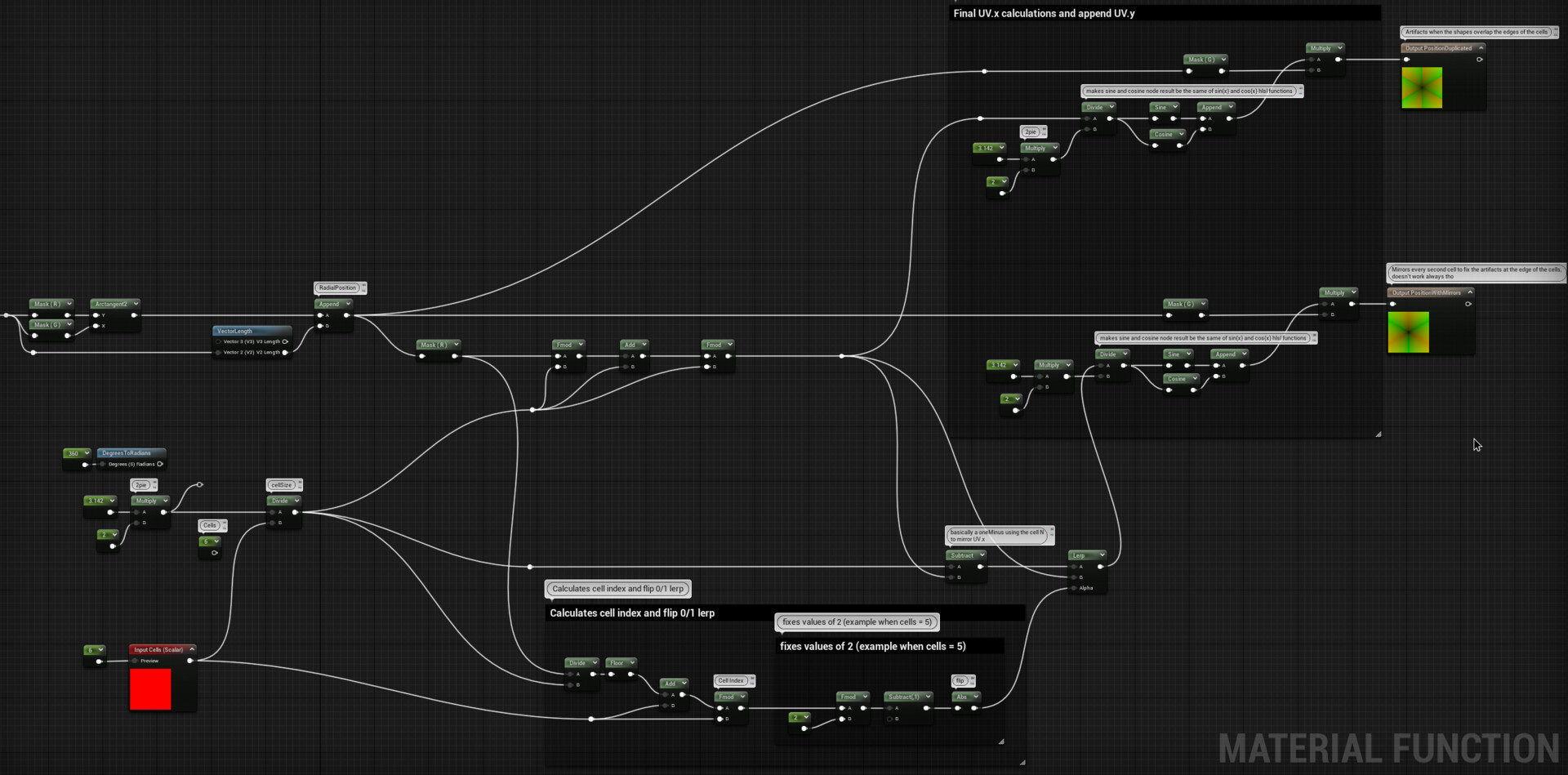
Regarding how to recreate it as an Unreal Function, like before, the function has two outputs, one for the duplicated position and the other one with the version with mirrors.

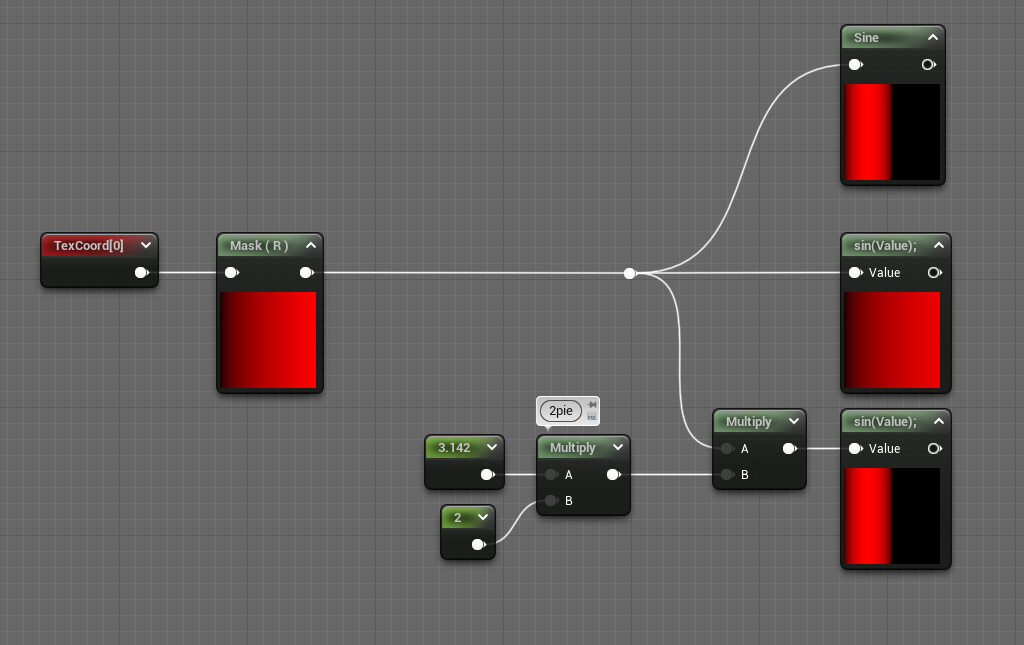
I need to mention that I've run into some complications when using Unreal's Sine and Cosine built-in nodes, I mentioned it in one of my previous posts as well. I realized that the input they take is normalized, so that when you feed a 0-1 value it outputs one wavelength. This makes these nodes a lot more useful and intuitive when using UV coordinates as inputs. However, the hlsl sin() and cos() functions to output one wavelength need 2pie as the input:

So, for the calculations we need in our function we need everything in radiants, so the hlsl function would give us the expected result.
However, you can find on Unreal's Documentation that using custom nodes "prevents constant folding and may use significantly more instructions than tan equivalent version done with built nodes", so for something simple like this I would try to avoid the custom node and instead try to get the same result using the built-in nodes.
In conclusion, this entire explanation was just to say that we need to divide by 2pie the inputs that go into our sine and cosine nodes, to recreate the same result of the hlsl functions.

The function is:

float radial_cells(input float2 Position, float Cells)
{
    const float PI = 3.14159;
    float cellSize = PI * 2 / cells;
    float2 radialPosition = float2(atan2(Position.x, Position.y), length(position));
    float cellIndex = fmod(floor(radialPosition.x / cellSize) + Cells, Cells);
    radialPosition.x = fmod(fmod(radialPosition.x, cellSize) + cellSize, cellSize);
    // Add this to make the version with mirrors
        // float flip = fmod(cellIndex, 2);
        // flip = abs(flip-1);
        // radialPosition.x = lerp(cellSize - radialPosition.x, radialPosition.x, flip);
    sincos(radialPosition.x, Position.x, Position.y);
    Position = Position * radialPosition.y;
    return cellIndex;
}

And here's the graph, where the sine and cosine inputs are divided by 2pie:

Here's the comparison of the two outputs, duplicated position on the left and mirrored version on the right:


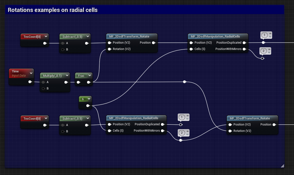
Rotation Examples

Like before, we can add some fun rotations and get different results based on if we do the radial mirroring of the UVs before or after the Rotate function.
For the sdf shape in these examples I've only used a triangle, with some offset to move the shape in the visible UV space:

The graph:

And here are the results,
rotation added before the mirroring:

Rotation added after the mirroring:


Library Examples

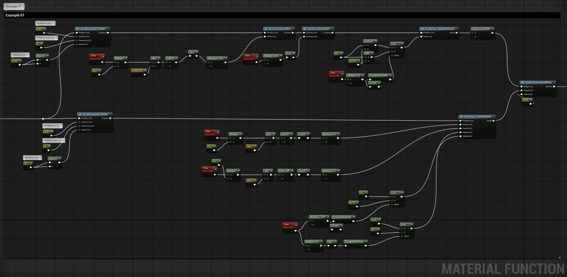
Here you can find a couple of examples of how to use together the sdf functions I've shown in these past 3 blog posts, to create some random morphing shapes.

For the first example, there are a couple of shapes floating around with their position animated and then merged together.


While this second one also has some shapes with their position animated, I've also added a mirror function to get a more complex result.


Conclusion

The next post will probably be the last one about this topic, I'll show how to make a flow map using a Sign Distance Field, which can then be used in the material to warp a texture or in Niagara to drive the location of particles. I'll also mention something about Anti Aliasing.
I hope you found this post useful, have a great rest of the day!

Report

2D SDF - Combine Shapes - Material Function Library UE5

Tutorial / 08 September 2022


Introduction

This is the second part of a series of posts about 2D SDF, check out the first one where I show some simple shapes and explain the basics to visualize them!
I think it's very useful and valuable knowledge for every Technical or Environment Artist, but really for anyone that works with materials.
In this post, I will cover ways to combine and merge these shapes, as well as share some extra tips I've learned along the way.
As I mentioned before, everything I will cover is not new knowledge, I've learned it all by reading Ronja and Inigo Quilez's articles which I highly recommend for getting a better understanding.
The focus of my posts is to show how their content can be recreated in Unreal Engine and its Material Graph.

I'm sorry again if this is another long post, but I hope it's worth reading, enjoy!!


Shape Morphing / Interpolate

I want to cover this first because, even if it's probably the simplest function, I think it's the more interesting and visually powerful.
Just by lerping between two sdf you can smoothly morph from one shape to the other.

float interpolate(float ShapeA, float ShapeB, float Alpha)
{
    return lerp(Shape1, Shape2, Alpha);
}

In the example below I'm lerping from a circle to a rectangle using a remapped sine wave as the alpha:


Combine Shapes

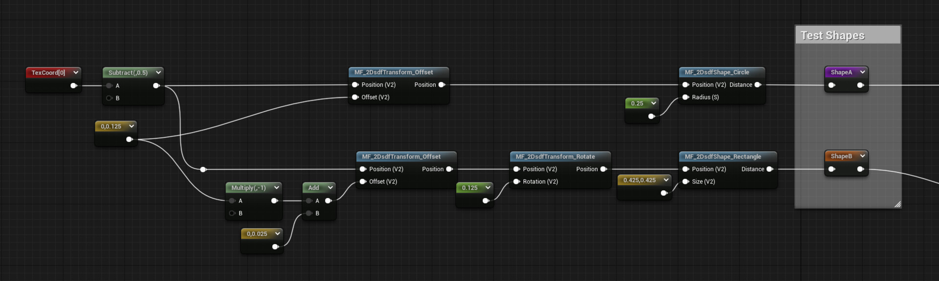
For this section, I'm going to use two shapes, a circle, and a square. The settings will always be the same so that the different results can be more easily understood.


Merge, Intersect, Subtract

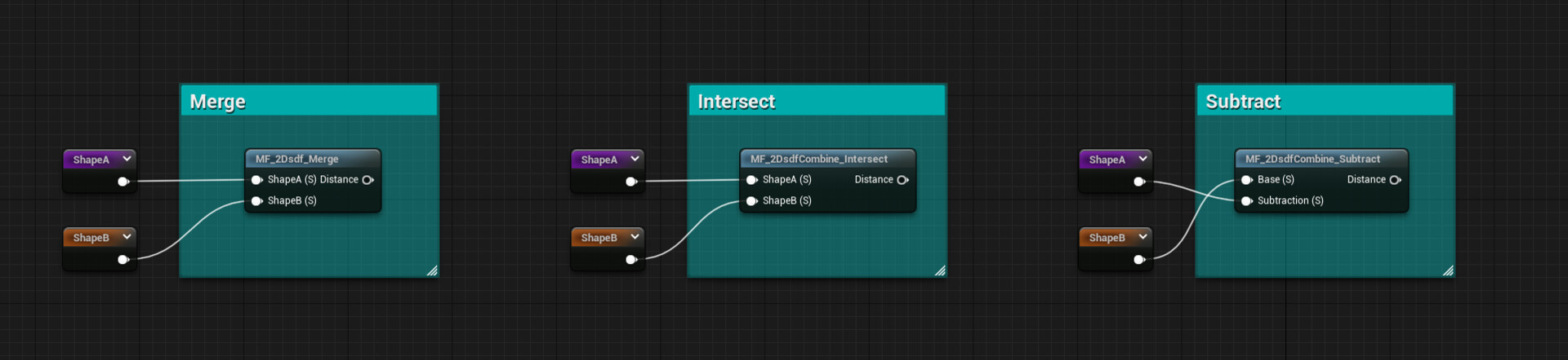
With some simple operations, the shapes can be merged, intersected, and subtracted from each other. There are 3 simple functions, but they are extremely useful to create more complex shapes.
Below you can see them in action:


Merge

The Merging result can be easily achieved with a Min operation:

float merge(float ShapeA, float ShapeB)
{
    return min(ShapeA, ShapeB);
}


Intersect

On the other hand, intersecting can be done using a Max node:

float intersect(float ShapeA, float ShapeB)
{
    return max(ShapeA, ShapeB);
}


Subtract

While a subtraction can be done using the Intersect function and feeding the subtracting shape after multiplying it by -1.
So it's essentially doing a Max operation but with one of the shapes inverted.

float subtract(float Base, float Subtraction)
{
    return intersect(Base, -Subtraction);
}


Rounded Versions

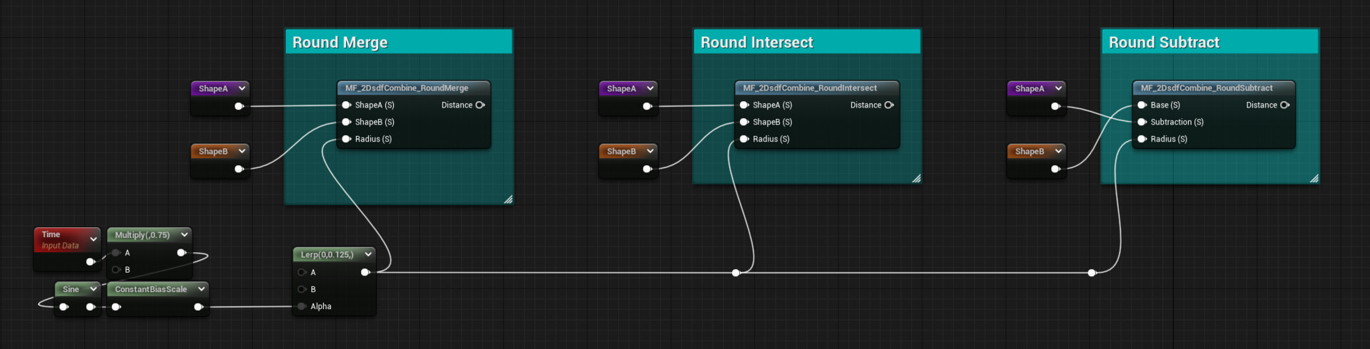
Using the functions shown before, we can create rounded versions as well, with control on the Roundness.
I'll try to explain them as best as I can but, If you want a more in-depth explanation of how this works, check out Ronja's tutorial.


Round Merge

By creating a vector2 using the sdf of the two shapes, getting the min value with 0 as the second input, and then the get its length, we can define an intersection Space. Then by growing the two shapes with a Radius parameter, the intersection becomes more rounded, but the two shapes are also getting bigger, which can be countered by subtracting the Radius again after the length function.
This gives us the result we wanted, but at this point, the sdf outside of the shape is currently broken, which can be fixed by doing the same operations but with inverted math to calculate the outside separately. Then two results can easily be combined for the output.

Here's the function:

float round_merge(float ShapeA, float ShapeB, float Radius)
{
    float2 intersectionSpace = float2(ShapeA - Radius, ShapeB - Radius);
    intersectionSpace = min(intersectionSpace, 0);
    float insideDistance = -length(intersectionSpace);
    float simpleUnion = merge(ShapeA, ShapeB);
    float outsideDistance = max(simpleUnion, Radius);
    return  outsideDistance + insideDistance;
}


Round Intersect

For the round intersect function the logic is the same, we just need to change a couple of things.
For the intersectionSpace we subtract Radius instead of adding it and we replace min with max.
We invert the length result for the inside distance and replace the Merge function with an Intersect one.

So that the function becomes:

float round_intersect(float ShapeA, float ShapeB, float Radius)
{
    float2 intersectionSpace = float2(ShapeA + Radius, ShapeB + Radius);
    intersectionSpace = max(intersectionSpace, 0);
    float outsideDistance = length(intersectionSpace);
    float simpleIntersection = intersect(ShapeA, ShapeB);
    float insideDistance = min(simpleIntersection, -Radius);
    return outsideDistance + insideDistance;
}


Round Subtract

For the Round Subtract function you can just use the Round Intersect one and invert the sdf of the subtraction shape:

float round_subtract(float Base, float Subtraction, float Radius)
{
    round_intersect(Base, -Subtraction, Radius);
}


Champfer Versions

Similarly, we can create a champfer at the transition points, with control on its position.

Champfer Merge

The champfer can be calculated by adding the sdf of the two shapes and dividing the result by the square root of 2, which it's the same as multiplying by the square root of 0.5. You probably already know this, but computers and software are faster at calculating multiplications rather than divisions (even if in this case it probably wouldn't really make a difference, I prefer using multiplication where I can).
To make things even faster, we could even feed directly the result as a float value, which is 0.70710678118. This way the shader doesn't need to calculate the square root at all.
After that, the champfer location can be controlled by subtracting a value from it, then by merging it with the 2 merged shapes it gives the desired result.

Function:

float champfer_merge(float ShapeA, float ShapeB, float ChampferSize)
{
    const float SQRT_05 = 0.70710678118;
    float simpleMerge = merge(ShapeA, ShapeB);
    float champfer = (ShapeA + ShapeB) * SQRT_05;
    champfer = champfer - ChampferSize;
    return merge(simpleMerge, champfer);
}


Champfer Intersect

For the intersection version, we just need to replace the simple Merge functions with the Intersect ones, and to control the location of the champfer we do an addition instead of a subtraction.

Function:

float champfer_intersect(float ShapeA, float ShapeB, float ChampferSize)
{
    const float SQRT_05 = 0.70710678118;
    float simpleIntersect = intersect(ShapeA, ShapeB);
    float champfer = (ShapeA + ShapeB) * SQRT_05;
    champfer = champfer + ChampferSize;
    return intersect(simpleIntersect, champfer);
}


Champfer Subtract

For the Champfer Subtract, like the Round Subtract, you can just use the Champfer Intersect function and invert the sdf of the subtraction shape.

Function:

float champfer_subtract(float Base, float Subtraction, float ChampferSize)
{
    return champfer_intersect(Base, -Subtraction, VhampferSize);
}


Groove and Round Intersection

Groove

This function creates a groove in one shape at the position of the border of another shape.
We need 4 inputs, the first two will take the sdf of the shapes, one will be the Base, while the other one will be the shape that drives the Groove location. The other 2 inputs are Width and Depth.
First, we subtract the Width from the absolute value of the Groove shape. Then we feed the result in the simple Combine Subtract function I showed earlier, and for the subtraction input of the function, we use the Base shape with the Depth added to it.
To get the final result we just need to use another simple Combine Subtract function, subtracting what we just calculated to the Base sdf shape:

float groove_border(float Base, float Groove, float Width, float Depth)
{
    float circleBorder = abs(Groove) - Width;
    float grooveShape = subtract(circleBorder, Base + Depth);
    return subtract(Base, grooveShape);
}


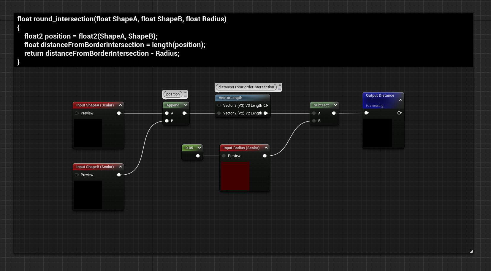
Round Intersection

This function, instead of combining the two shapes using boolean operations, creates new round shapes where the borders of the two sdf overlap.
To achieve this, as I showed in the Round Merge function, we need to define the Intersection Space by interpreting the two shapes as the X and Y axis of vector2, this way the intersection points will be coordinate 0;0.

Then, as we do for a simple circle shape, we can create rounded shapes by calculating the distance from the origin and subtracting an arbitrary value to control the Radius:

float round_intersection(float ShapeA, float ShapeB, float Radius)
{
    float2 position = float2(ShapeA, ShapeB);
    float distanceFromBorderIntersection = length(position);
    return distanceFromBorderIntersection - Radius;
}


Conclusion

The next part will be about manipulating, in more advanced ways, the coordinate space used to sample the SDFs.
I hope you found this post useful, have a great rest of the day!


Report

2D SDF - Basic Shapes and Visualization - Material Function Library UE5

Tutorial / 01 September 2022

Introduction

I've been working on a Material Function Library for 2D Sign Distance Field that contains shapes and relative merging and manipulating operations.
I think it's very useful and valuable knowledge for any Technical or Environment Artist, but really for anyone that works with materials.

There will be a few posts about this topic, in this first one, I will show how to make some simple shapes and explain the basics to visualize them.
I will then cover different ways to combine these shapes, more advanced techniques to manipulate them and then how you can use distance fields to create gradients and flow maps.
Everything I will cover is not new knowledge, I've learned most of it by reading Ronja and Inigo Quilez's articles which I highly recommend for getting a better understanding.
The focus of my posts is to show how their content can be recreated in Unreal Engine, as well as share some extra tips I've learned along the way.

I'm sorry in advance if these posts will be long, but I think they are worth reading, enjoy!!


Basic Shapes

Let's start with some basic shapes, the screenshots and gifs you will see below are using a function I made that helps visualize distance fields.
For now, all you need to know is that the thicker white line represents the SDF shape, red is for the inside, and light blue is for what's outside of the shape.

One thing that all the shape functions share is that they require a Position input, to keep things simple I'm just using the UVs and then visualize the result on a simple plane. To center them I just subtract 0.5 from the UVs, I didn't include the subtraction node in the functions themselves so that they are more versatile and can be used, for example, with Wolrd Position values.

Circle

This is for sure the easiest distance field function:

float circle(float2 Position, float Radius)
{
   return length(Position) - Radius;
}
[snippet]

The size of the circle can be controlled with the Radius parameter.


Rectangle

Here's the rectangle's function:

float rectangle(float2 Position, float2 Size)
{
    float halfSize = Size * 0.5;
    float2 d = abs(Position) - halfSize;
    float outsideDistance = length(max(d, 0));
    float insideDistance = min(max(d.x, d.y), 0);
    return outsideDistance + insideDistance;
}
[snippet]

Size can be controlled with a vector2, this allows independent control on the 2 axes or just input the same value for both to get a square.


Triangle

The triangle's a little bit more complicated:

float EquilateralTriangle(  in vec2 p, in float r )
{
    const float k = sqrt(3.0);
    p.x = abs(p.x) - r;
    p.y = p.y + r/k;
    if( p.x+k*p.y > 0.0 ) p=vec2(p.x-k*p.y, -k*p.x-p.y) / 2.0;
    p.x = p.x - clamp( p.x, -2.0*r, 0.0 );
    return -length(p) * sign(p.y);
}
[snippet]

Similar to the circle, the size can be controlled with a single float.


Segment

The segment's also another very useful shape:

float Segment( in vec2 p, in vec2 a, in vec2 b )
{
    vec2 pa = p-a, ba = b-a;
    float h = clamp( dot(pa,ba)/dot(ba,ba), 0.0, 1.0 );
    return length( pa - ba*h );
}
[snippet]

This function actually draws a line between two points, so the inputs are two vector2 parameters, and each vector2 defines the location of one of the points.
Regarding the thickness of the line, it's not defined by an input but it can still be adjusted by using another technique explained below.


Rounded Corners

Each point in a distance field only stores one value: the distance to the closest point of the perimeter of the shape we're representing. You probably noticed on the images and video shown above that the lines "outside" of the shapes are getting rounder and rounder the further away they are from the shape perimeter. If you go far enough any distance field becomes a perfect circle.
This can be used to our advantage, subtracting a value to the SDF before visualizing it will round the edges of any shape, this is also how I changed the thickness of the Segment shape earlier.

The only thing you need to be aware of when doing this is that in the process of rounding the edges the shape also changes in size and becomes bigger since now to visualize the shape we're essentially using points further away from the original perimeter.
So, you will have to scale it down if you wanted the shape to remain of the previous size. I'll cover both visualization and scaling methods later in the post.

The following graph and the video shows an example of a square SDF in both its original and rounded state, trying to keep them both the same size.

Here's a comparison of the graphs:

  • Basic Shape
  • Rounded Edges
  • Rounded Edges with Scale Compensation


Basic Visualization Methods

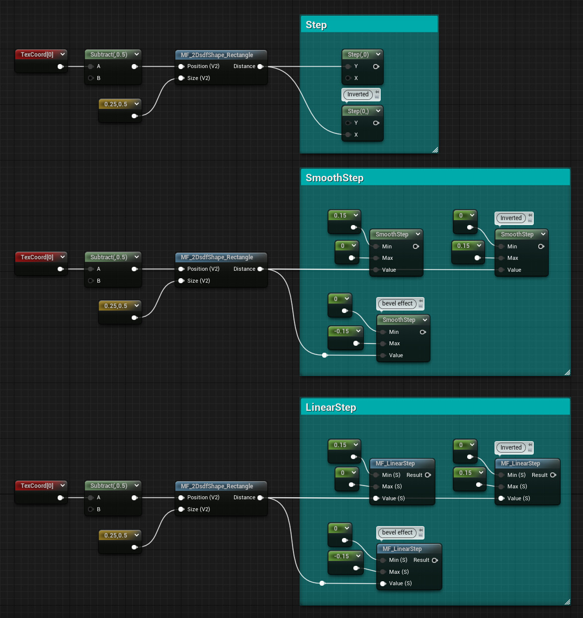
I would say there are 3 basic methods to visualize sign distance fields, which involve Step, Smooth Step, and Linear Step functions.
If you want to learn more about them you can check out one of my previous blog posts where you can find more information about them.

Step

The most straightforward and basic way to visualize a distance field.
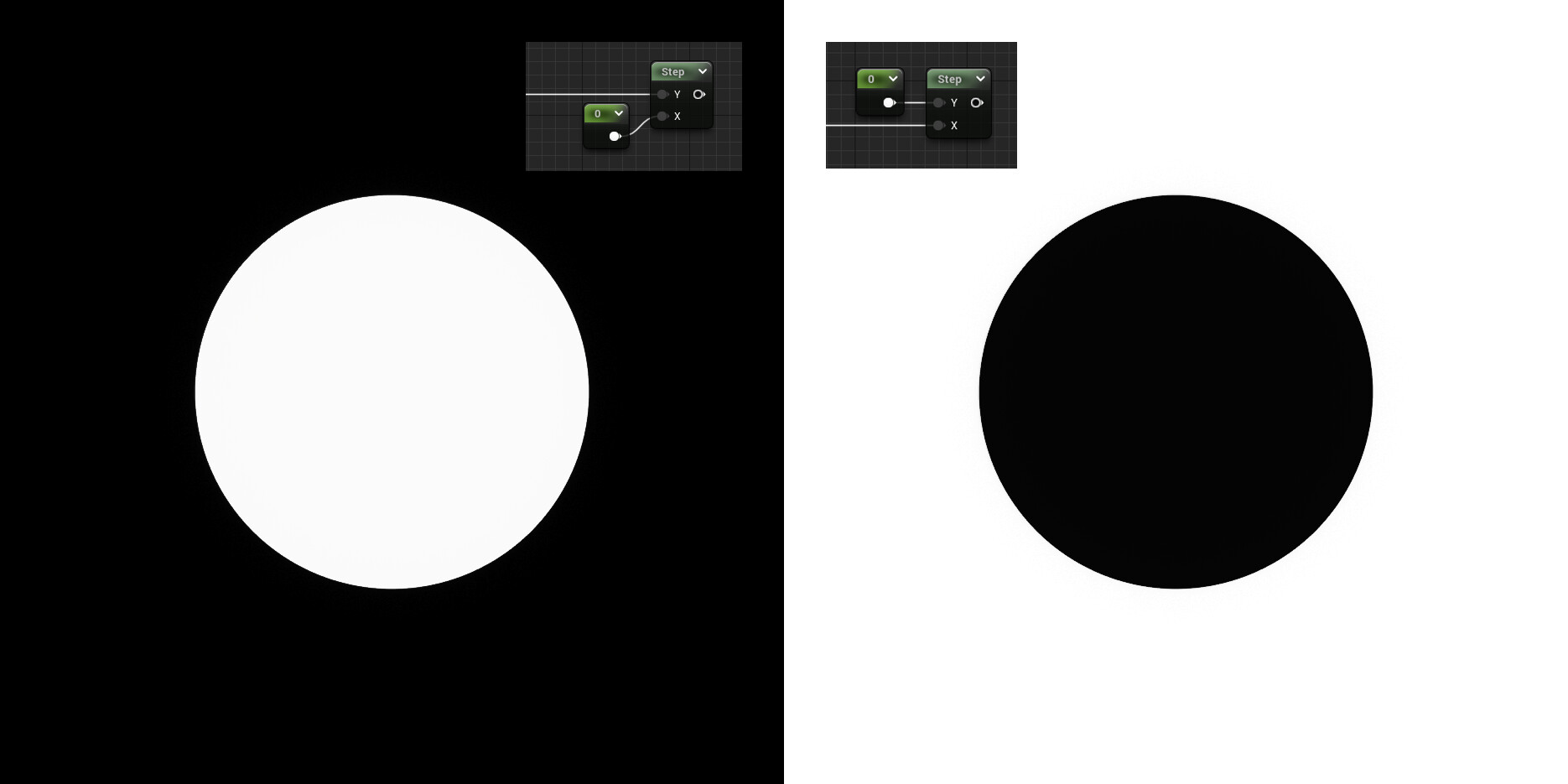
Simply drop a step node, and use the SDF as the first input and a value of 0 as the second input. If you want to invert the inside and outside of the shape, just invert the two inputs.


Smooth Step

The Smooth Step it's probably the function I use the most to visualize SDF because It creates a nice gradient and you can define its start and end position.
Similar to the Step function, you can invert the Min and Max value to invert the inside and outside of the shape.
The example below shows a Min value of 0.1 and a Max value of -0.1. This makes the gradient start where values are -0.1 in the SDF, which are inside the perimeter of the shape, and it ends where the values are 0.1, just outside of the perimeter.


Linear Step

The unwanted and a little bit ugly brother, it's exactly the same as the Smooth Step function, the only difference is that the interpolation is linear instead of smooth. I've never really found it very useful, but I wanted to mention it there since it might be a good option in some specific cases.
Of course, there isn't a built-in node for it in Unreal's Material Graph, so you will have to make your own function, again, more about it here.


The screenshot below gathers all methods in one image.
Using values inside the perimeter of the shape for the Smooth Step and Linear Step functions also gives an interesting result, something similar to a bevel node in Substance Designer.


Animate Shapes

As you noticed in the videos above, the shapes can be animated. That can be easily done just by animating the parameters using time nodes and sine and cosine functions, the shapes will automatically update.

Below you can see a couple of examples.
For the Circle I'm using a Sine node and ConstantBiasScale to remap the value between 0 to 1, then I just used the result as the Alpha value for a Lerp, this way I can easily control the min and max value of the animation. Time is also multiplied by a float to control the speed.
In the Rectangle example, since it needs a vector2 and I wanted the animation of the 2 values to have an offset I've added an arbitrary value to one of the two and then did the same as before, but using a cosine instead of sine. Because the output it's a vector2 I can't use it directly as an Alpha for a lerp to do control the animation, so instead, I remapped the values using a multiply and an add node, essentially creating a "ConstantScaleBias" having the multiply control the overall size and the addition node to offset the animation away from 0 (different from BiasScale since the two operations are swapped). Again, Time is multiplied by a float to control speed.


Annular Shapes

SDF can be visualized in a way that gives annular shapes.
All the values outside of a shape are positive, while the ones inside its perimeter are negative.
This means that if we absolute the SDF so that we only have positive values we're left only with the perimeter of the shape, where the values are 0. If we then subtract from it we can make all the values near the perimeter negative, creating annular shapes. The subtraction amount controls the thickness of the shape.


Waves Patterns

The SDF can be used to create some interesting wave patterns, I'll cover them now.
Frequency can be controlled by multiplying the SDF. In all the examples, I'm also adding time to animate them.


Frac

Returns the fraction part of the SDF. You should get the same result using a % node and value of 1 for the second input.


Sine and Cosine

Of course, they both give basically the same result, the output will be a gradient that goes between -1 and 1, if you want only positive values you can try an abs or ConstantBiasScale node.


Triangle Wave

Very similar to the previous example, but it returns a linear gradient.
Check out one of my previous posts about it.
In the example below the gradient goes from 0 to 1.


Smooth Stepping Curve

I tried to experiment with this function as well.
You can find more about it here to use it in Unreal Engineand here if you're interested in it for remapping noises in Substance Designer.


Other - Tangent

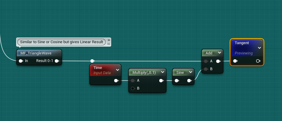
I wanted to share a couple of more interesting findings using tangent nodes.
The first one is just using the tangent after a ConstBiasScale of a Sine node:

The second one is a little bit more trippy, this is the setup:


Advanced Visualization

If you've read everything up until here you are now ready to create your own custom advanced visualizer like the one you saw earlier.
You can use positive and negative values to colour the inside and outside of the shape, use the annular technique to visualize its perimeter, wave patterns to show the outer and inner space distances and use Smooth Step functions to create some nice subtle shadow gradients.
Here you can find the snippet of the one I made, but I highly recommend you try and make your own one, it's a fun challenge!


Basic Transformations

One last thing I wanted to cover in this post is how SDF can be manipulated using basic transformations such as offset, rotate and scale.
The way this is done is by transforming the position values that are fed in the SDF Shapes functions.

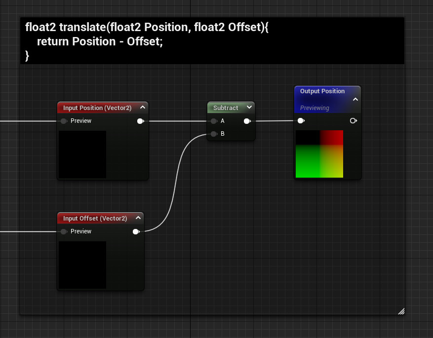
Offset

The offset is quite simple, just subtract from the Position. We're not doing an addition because we are manipulating the space. If we move the space towards a direction, the shape we draw into it will move the opposite way.

float2 translate(float2 Position, float2 Offset)
{
    return Position - Offset;
}


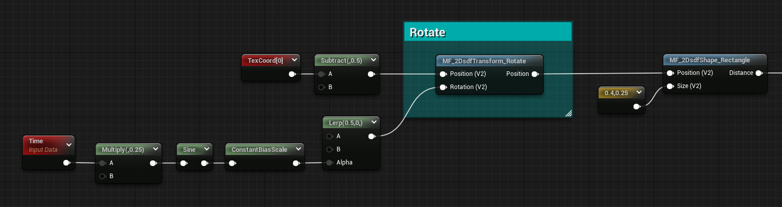
Rotate

The rotation's definitely worth having inside a function, unlike offset and scale.

I noticed some weird behavior from both the Sine and Cosine nodes in Unreal, they don't output the same value sin() and cos() do in hlsl. To get the same result you need to divide the input of the nodes by 2pie. I think this was done to make the nodes give better out-of-the-box results when TexCoord and Time nodes are plugged in as the input.
So unlike Ronja, to have the rotation being from a 0 to 1 value I didn't have to remap it to radiants. I found this very interesting since this affects any rotational math done in the material graph, so I've left the nodes inside a comment for future reference.

float2 rotate(float2 Position, float Rotation)
{
    float sine = sine(Rotation);
    float cosine = cosine(Rotation);
    return float2(cosine * Position.x + sine * Position.y, cosine * Position.y - sine * Position.x);
}


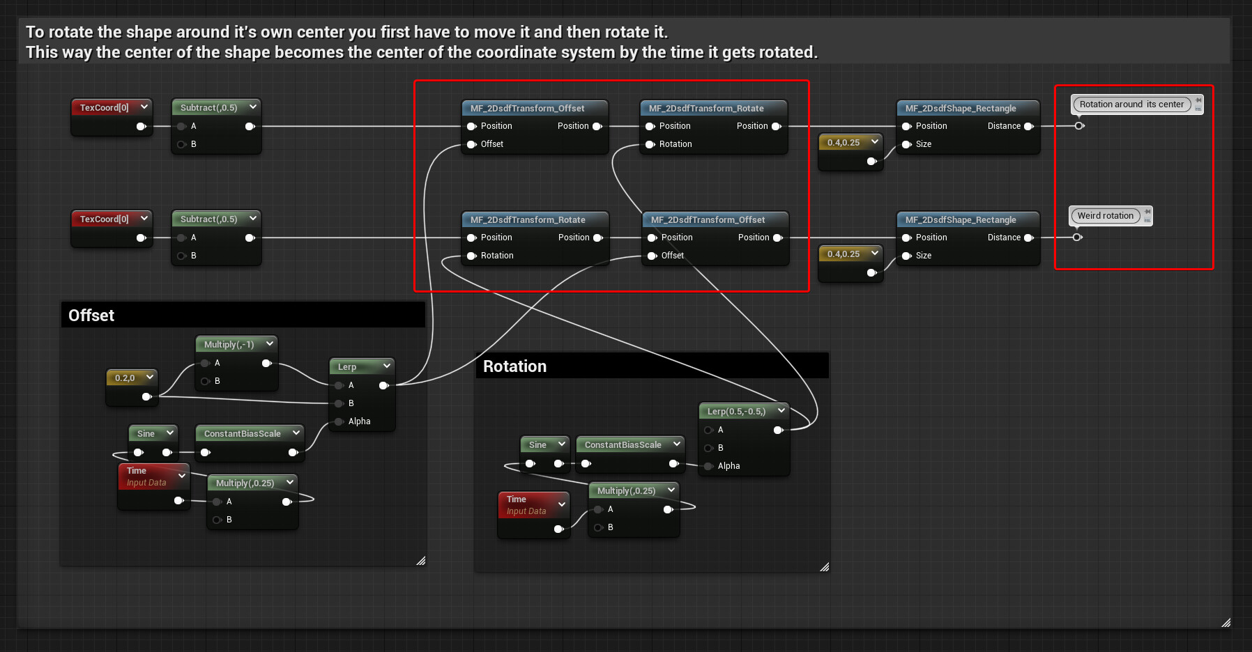
Another thing to mention is that if you're using both Rotate and Offset functions, the order you use them gives different results. If you want the shape to always rotate at its own center the Rotate function should be used after the Offset one.
Below you can find a comparison, when the rotation is done before the offset the result it's weird, but might be desired in some cases.


Scale

You might find this a little bit useless since most of the SDF Shapes functions I showed you at the start of this post have already controls for their size. However, when you have multiple of them and start using some merging functions this is a quick way to rescale them all at the same time.
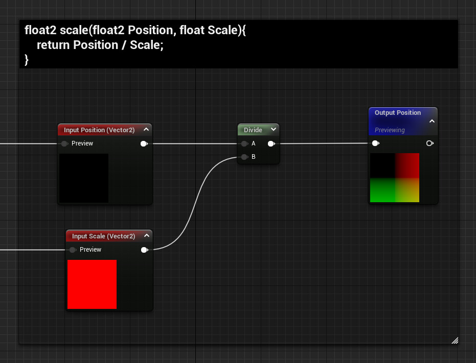
The function's simple, get the position and divide it by the scale.

float2 scale(float2 Position, float Scale)
{
    return Position / Scale;
}


Conclusion

If you didn't realize it yet, I fell in love with distance fields and I hope you can now see their potential as well!!
However, if that's not the case and you're still resisting their magnificent charm, don't worry, there will be a few more posts about them that will cover more advanced techniques!

I know this post was quite long, but I really appreciate you've read the entirety of it!!
(Eheh yes, I'm looking at you scroller, you should feel ashamed, go back up and look at all the pretty pictures at least!!)
Jokes aside, thanks a lot, I hope I managed to teach you something new, have a good rest of the day!

Report

Copy To Points Randm Input - Houdini

Tutorial / 18 August 2022


Introduction

Here's a very simple but quite useful tip for Houdini, let's say you are working on a landscape and you want to scatter some random rocks on it, in this post I'll show you how you can do that!
To achieve this we need to give a unique ID attribute for each object you want to scatter and then use a Copy to Points node.
In the example I'm going to show you, the unique ID will be called variant.


Objects Pool

Let's start with putting together all the objects we want to randomly pick from, creating an "Object Pool" that we can use later to reference the objects from.
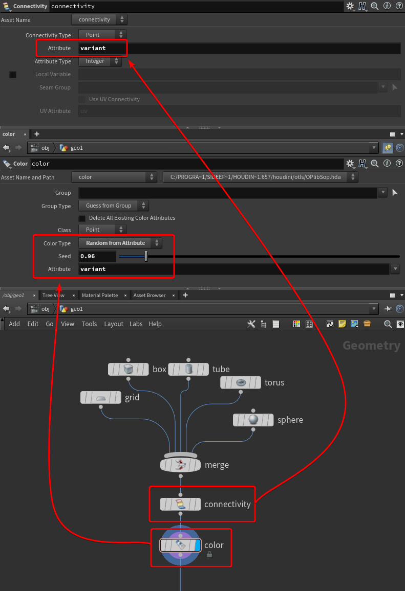
The only thing we need is to give them a unique integer attribute. If all the objects are made out of single meshes then we can easily use a Connectivity node.
In the example below I used this node, only changing the default name it creates from "class" to "variant", and then I'm driving a color node to pick a random value using this attribute:

However, if your object is composed of multiple meshes, like Houdini's test geometry Rubber Toy is,  this won't work since the Connectivity node creates the attribute for each set of connected primitives or points.
You would get this result instead:

I found two alternatives to this problem, but please reach out if you know a better way of doing this.
The first method is a little bit manual, you can create and set the variant attribute on each object before they get merged, but this means you have to type the various numbers one by one and edit them by hand if you add or remove objects:

The other alternative is to use the Pack node before merging, and the Unpack one after creating the variant attribute.
The only thing to remember when using Pack and Unpack nodes is that by default it doesn't keep any of the attributes or groups your geometry has, so just remember to use the Transfer option of these nodes accordingly. You can just type an asterisk to select all the attributes the mesh has, and do the same for the groups if needed.

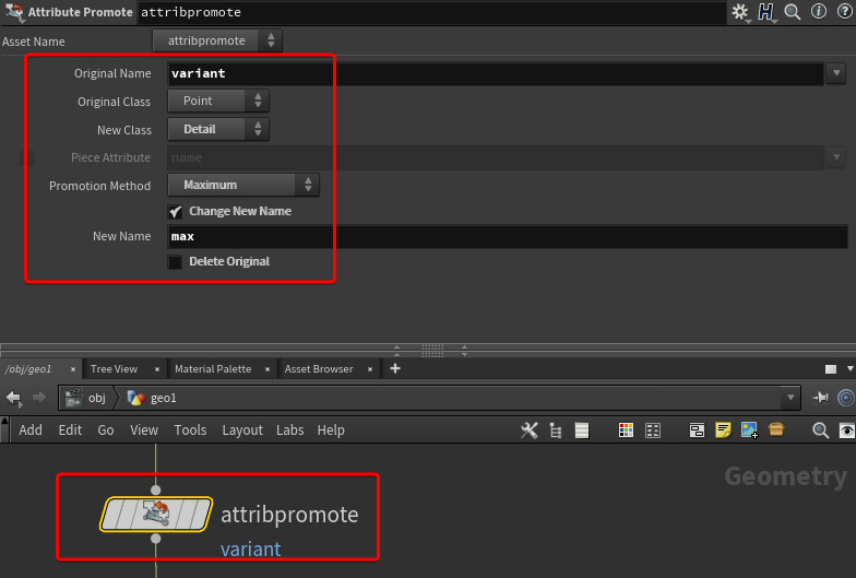
Once that's done we need to create another parameter that tells us how many different objects we gathered together, which will be needed for the next step.
We can easily to that with the Attribute Promote node, just change the Promotion Method to Maximum, I'm also storing this information as a Detail Attribute and renaming it to "max".


Target Points

Now we can finally start defining the points we are going to copy these objects into.
For this example, I'm just using the points of a simple grid, the only thing we need to do is to assign a unique ID for each of these points, which will correspond to the different objects in our Pool.
I'll show you two different ways of doing it, one with VEX and the other one just using built-in nodes, however they both use a neat technique to reference our Objects Pool node, more specifically, we need to read the max Detail Attribute we made earlier.

Spare Input

We can add a Spare Input to any node you want, just select your node and add one from the menu the cog icon opens. A "Sapre Input 0" Parameter will be added.

Now if you drag and drop the Object Pool node into the Spare Input slot a purple dotted line appears, which means we can now reference it directly.


The two methods

The first method I'll show you uses two built-in nodes
First create an Attribute Randomize, change the Attribute Name to "variant" and under the Distribution tab set it to "Uniform (Discrete)" (to get only whole numbers) and for the Max Value we want to reference max attribute from the Objects Pool,  since we created that purple connection earlier we can simply write:

detail(-1, "max", 0)

Because the surface node -1 it's the Spare Input 0

Under the Options tab you can also change the seed.
Now the only problem is that the attribute created it's a float, but we need it to be an integer, to convert it we can use an Attribute Cast, just write the parameter's name and change the Precision to 16-bit integer.


For the VEX alternative, we can run over the Points using an Attribute Wrangle:

i@variant = set(rint(rand(@P + chi("Seed")) * chi("Amount")));

In this case, I'm driving the randomization using the point's position and adding a float as a seed. However the rand function gives a value between 0 and 1, but we need a value between 0 and the max amount of objects we have in our Pool, to get that value we can reference it the same way as I showed before.
One last thing to note is that the rand function will give us a decimal numeral, using set() we can explicitly tell Houdini to convert the float to an integer, but that will only truncate the number, which means we'll never get the last variant ID of the Pool. To include it, we'll have to round the number using rint().


Final Step and Last Notes

We are finally ready to put together the Pool with our Points with a Copy To Point node, we just need to turn on Piece Attribute and select our attribute variant.


Here's the result with our beautiful graph:

Randomize the result with the seed parameters mentioned earlier

I hope you found this useful, have a great rest of the day!!

Report

Perfectly Remapping a Cube to a Sphere - Houdini

Tutorial / 04 August 2022


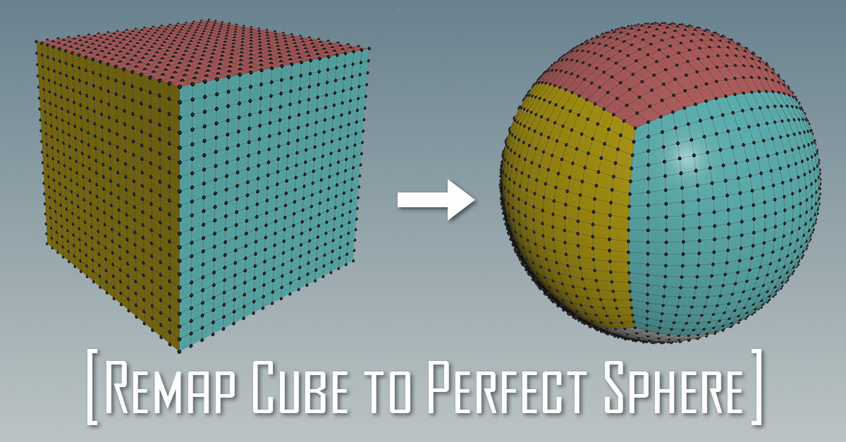
A perfectly rounded sphere, with clean and uniform topology. I'm sure every artist that works with 3D models needed something like this at some point.
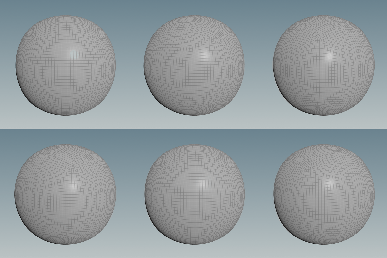
We all went down the route of subdividing a cube multiple times, but that doesn't translate to a perfect sphere:


A good workaround would be to reproject the geometry of the subdivided cube to a normal sphere, triangulated, with pinches at the poles or just having it as a Primitive.
The gif below shows a comparison animation of before and after the projection:


In Houdini it can be done using a Ray node, both the Project Ray and Minimum Distance options give similar results, you just need to make sure you scale the subdivided cube accordingly. For the minimum distance, you can get better results if the two surfaces match as close as possible, on the other hand, to make the ray option work the subdivided cube surface needs to be fully encapsulated by the sphere (or the other way around if you invert the rays' direction), but they should still be of similar size for a better result.
Below you can see the sizes of the spheres for the two different setups: 


If you can't be bothered to set it up yourself and have the Labs Tools installed, you can use the Labs Sphere Generator node, it uses this technique with Ray's Method set to Project Rays and it also generates UVs.


This helps however, the sphere you get is not completely accurate since it's dependent on the resolution and frequency of both the subdivided cube and the projection sphere used.
Here's when we turn to our friend maths and ask if it can fix our problems.
It can help us out transform a cube into a perfect sphere. We can do it using a Normalize function, applying it to the vector position of each point will cause all the points to be the same distance from the center.
This happens because it divides the vector by its own length, here's the code in VEX of three ways to achieve the same result:

@P = normalize(@P);

@P /= length(@P);

@P /= sqrt(@P.x * @P.x + @P.y * @P.y + @P.z * @P.z);


To increase the resolution of the cube you can simply use a Subdivide node with the Algorithm set to "OpenSubdiv Bilinear", but I found you can have more control in creating the cube from a Plane (Grid node in Houdini), this way you can specify exactly the resolution with a number.
You can do it using some Transform and Mirror nodes, at this stage you can also set up the UVs and assign a random colour to each face using the Connectivity node before fusing the points together.


However, the method showed above still bothers me because you can see that the vertices in the area of the original cube's corners are a lot closer to each other compared to the ones at the center of the cube's faces.


Luckily someone came up with a fancy equation that maps the cube to a sphere keeping the points spread out more evenly, almost as if you're relaxing them.
The function is:


In VEX:

float x2 = @P.x * @P.x;
float y2 = @P.y * @P.y;
float z2 = @P.z * @P.z;

@P.x = @P.x * sqrt(1 - (y2 / 2) - (z2 / 2) + (y2 * z2) / 3);
@P.y = @P.y * sqrt(1 - (z2 / 2) - (x2 / 2) + (z2 * x2) / 3);
@P.z = @P.z * sqrt(1 - (x2 / 2) - (y2 / 2) + (x2 * y2) / 3);


The gif below shows an animated comparison of the points using the two methods:

I find this animation very satisfying to look at, I can finally sleep again at night.

I hope you found this post useful, have a great rest of the day!!


Report

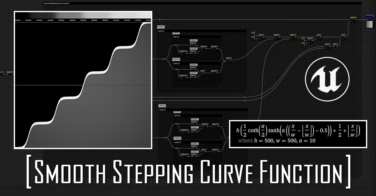
Smooth Stepping Curve Function - Remap Noises for stylized look - Unreal Engine

Tutorial / 07 July 2022


A month or so after making the Smooth Stepping Curve Function in Substance Designer, I wondered if the same could be done in Unreal Engine.
Turns out you can, but each function does add 22 instructions to the material.
I don't think I will use it much in the future and I don't really advise it for production projects, especially because in Substance Designer I found I could get better results pairing it with a blurring node (more about it here), which is not really an option in Unreal's Material Graph. For this reason, I prefer just exporting the texture directly out from Designer.

Here you can find the function applied to 3 different noises


This is the texture I used if you are interested:
Red Channel - Clouds 2
Blue Channel - Perlin
Green Channel - Crystal 2
(Substance Designer noises)


The function can be visualized and debugged by applying it to a left to right, 0-1 gradient, simply using the Red channel of the "TexCoord" node.
Then the remapped gradient can be put into a visualizer, you can find the one I made here, in there I also show the basics needed for making your own one.


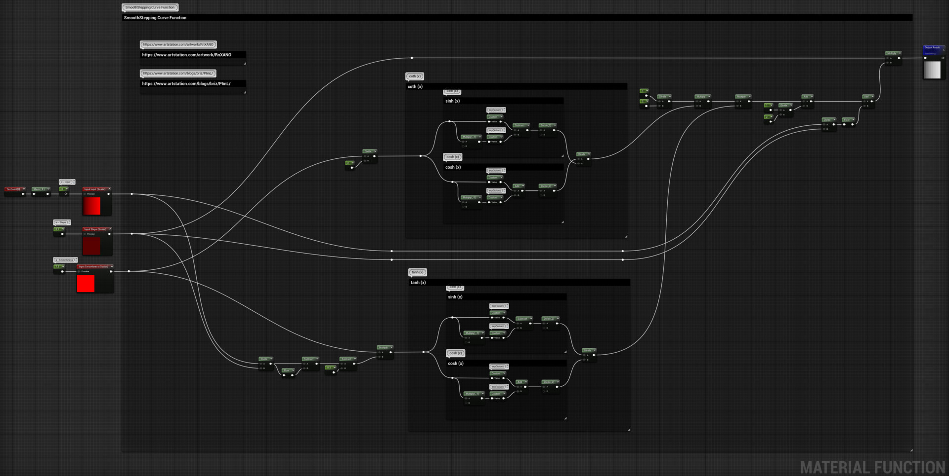
Something to mention, I don't think Unreal's Material Graph has a node for the Exponential function, so unfortunately I had to use custom nodes for it:

exp(Value);

This is the function's graph:

You can find the snippet here on Unreal's Forum.

Thanks for reading!!

Report